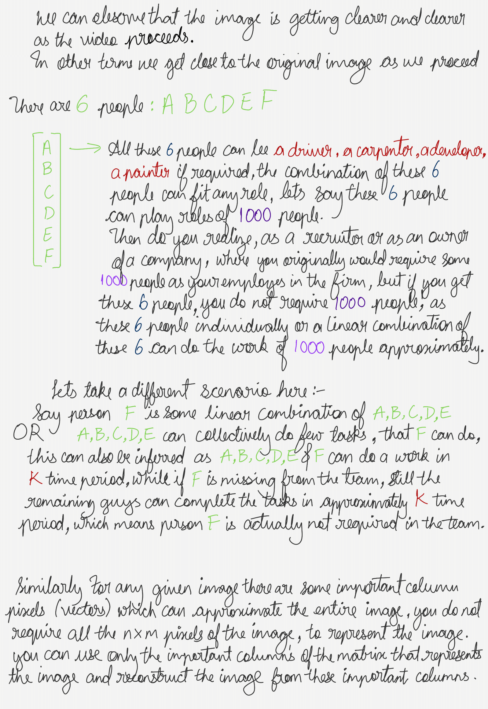
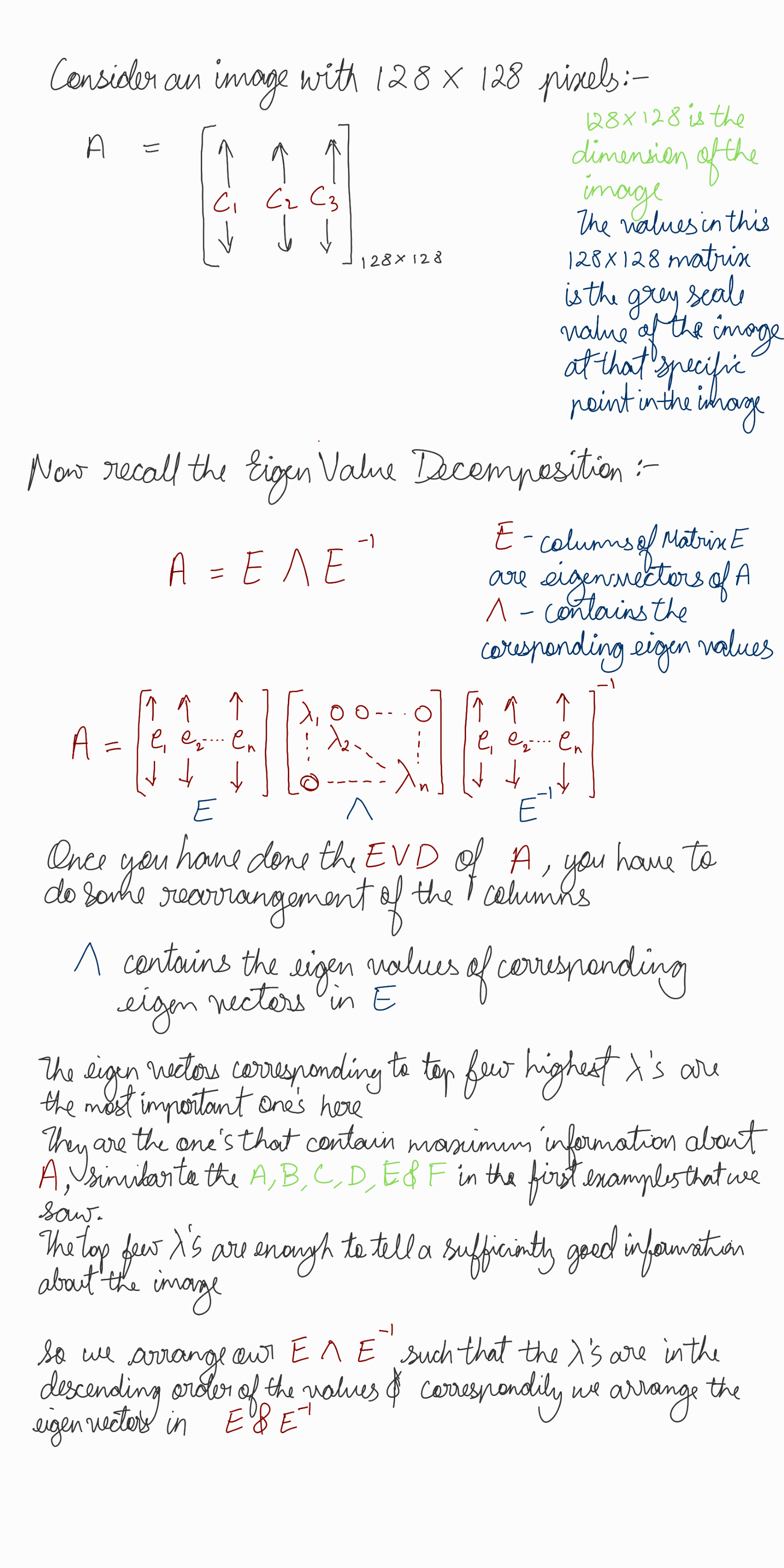
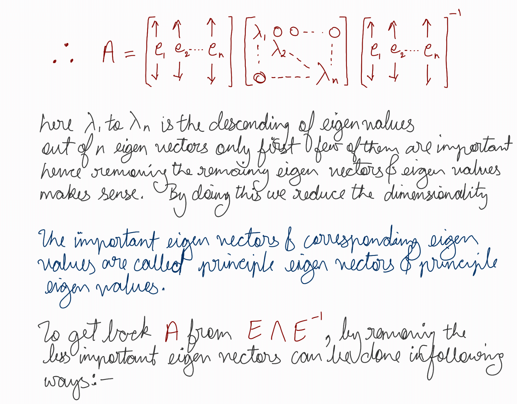
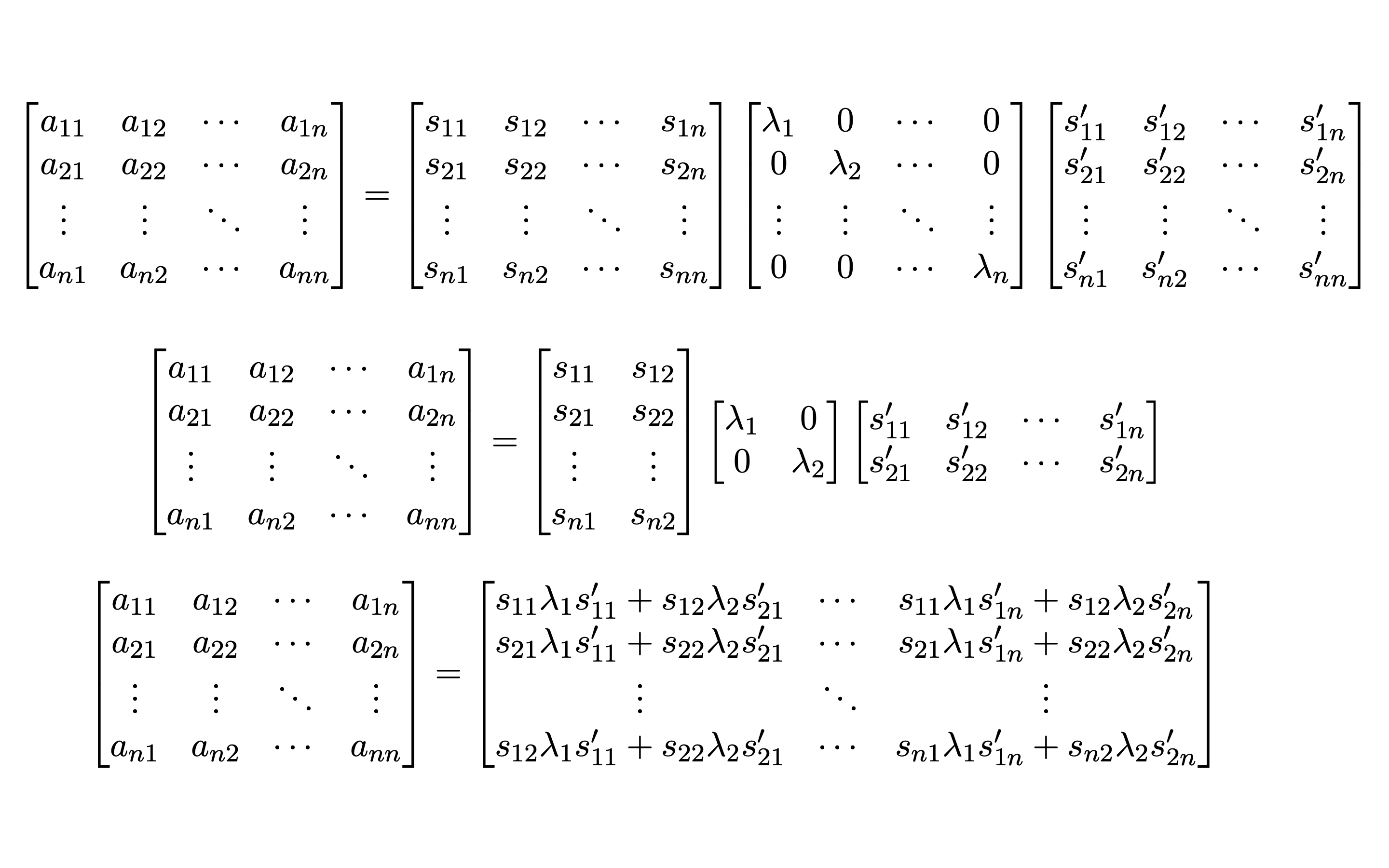
Galaxy
- Motivation for ML
- Markov Processes
- Taylor Series
- Gradient Descent
- Least Squares
- QR Factorization
- Hoeffding’s inequality
- Perceptron Learning Algorithm
- SVD
- The Learning Problem
- SVM
- Introduction to Clustering
- K-Means Clustering and Lloyd’s Algorithm
- Convergence of the K-Means Algorithm
- Nature of Clusters Produced by K-Means
- Initialization of Centroids in K-Means and K-Means++
- Choosing the Number of Clusters \(K\) in K-Means
- Learning From Data
- Lady Tasting Tea
- Neural Networks
- Lecture-11/11/2024
Motivation for ML
HES-Subjects Example
Let’s start with a simple question: Given the marks of a student in English and Hindi, can we predict the marks they might get in Sanskrit? What if we try to see it as a linear combination?
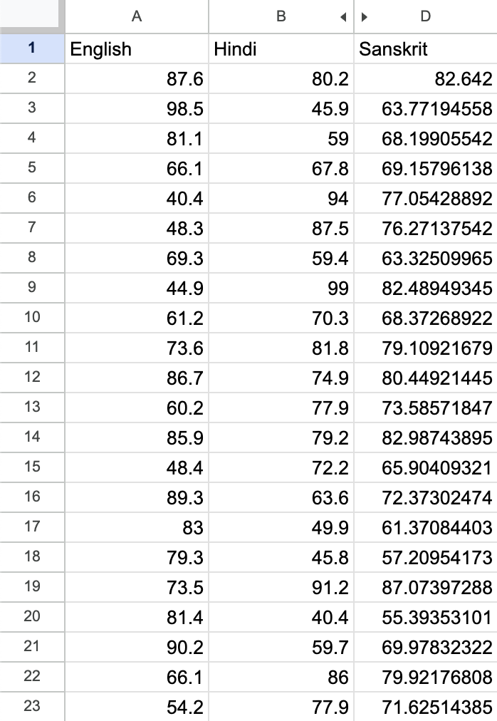
Think about it like this — can we find a combination of English and Hindi marks that equals the Sanskrit marks? For example, could it be that:
0.2 * English + 0.8 * Hindi = Sanskrit- Or maybe
0.6 * English + 0.4 * Hindi = Sanskrit?
Now, here’s something to ponder: we only looked at two subjects, but what happens if we throw in more subjects? What if we have 3, 4, 5, or even 100 subjects? Do you see how the complexity of this question ramps up significantly?
As the number of subjects increases, it becomes harder and harder to find the right combination. The challenge here is to figure out if we can express the marks in one subject as a linear combination of the others. How would you approach this problem when dealing with multiple subjects?
Radio Example: Parameter Tuning
Let’s take a trip back to the 1930s. Imagine you’re tuning an old radio with a knob controller. To find the right station, you’d have to slowly tweak the knob, trying to tune into the clearest signal. So in a way, you were performing an algorithm to connect to the best station.
Now, what do you think happens when you turn the knob clockwise? What if you hear loud noises? Naturally, you’d switch direction and try turning it anticlockwise, right? And if you start hearing faint music, you’d keep turning in that direction to zero in on the best sound.
This is very similar to what we do in Machine Learning. We try to tune our parameters to reduce noise or loss and increase the score. Can you see how this old-school radio tuning is just like parameter tuning in ML?
You start with one direction, assess the output (in this case, the sound), and then decide whether to continue or adjust your approach. The goal is always to find that sweet spot where everything sounds just right, or in ML terms, where the model performs optimally.
Binary Search: The Laptop Thief
Imagine you’re given a 4K resolution video that runs for 4.5 hours. The video shows a study table, and at the beginning, there’s a laptop on the table. But by the end of the video, the laptop is gone—someone has stolen it. Here’s the challenge: you need to find the exact moment when the laptop was taken. But watching the entire 4.5 hours of footage seems impractical, doesn’t it?
What’s the best way to tackle this?
A smart approach would be to jump to the middle of the video and see if the laptop is still there. If it is, then the theft must have occurred in the second half. If it’s not, then the first half is where the action happened.
What would you do next? You’d continue this process, checking the middle of the relevant section each time until you pinpoint the exact moment when the laptop was picked up.
Why is this method so efficient? It’s because you’re using a binary search technique, which allows you to find the moment in log(n) time. Instead of scanning through every second of the video, you’re drastically cutting down the time it takes to find the key moment. Can you see why this method is so powerful?
COVID Testing: Minimizing the Number of Tests
Consider a scenario where a clinic needs to test a group of 10 people for COVID-19. Individual testing is expensive, so the clinic needs an efficient strategy to minimize costs. How can they do this?
The best approach is to minimize the number of tests while still accurately identifying infected individuals. Here’s how it can be done:
- Initial Batch Testing: The lab assistant divides the 10 test samples into two groups of 5. She then mixes the samples of each group and tests them in two separate test tubes.
- If the first batch tests positive, she knows that someone in this group is infected. The second batch, which tests negative, can be ignored—saving 5 tests!
-
Further Subdivision: Now, the assistant takes the positive batch and divides it into smaller groups, perhaps 2 and 3 samples each, and tests them again. By following this process, she narrows down the infected individual(s).
- Efficiency: This method is highly efficient because it halves the search space in every iteration. The assistant only conducts the minimum number of tests necessary to identify the infected person(s).
Can you figure out the minimum number of tests required for any number of samples, \(n\)?
It’s log(n). This is where you can see the binary search in action!
To make it even more efficient, you could experiment with different batch sizes, like grouping \(k\) samples together instead of just 2. This could further reduce the number of tests required.
Finding \(\sqrt{11}\)
Finding the square root of 11 is equivalent to finding the root of the equation
\[x^2 - 11 =0\]Note that one can observe that the root lies between 3 and 4, simply because considering \(f(x) = x^2 - 11\), \(f(3)<0\) and \(f(4)>0\).
This means the answer lies between 3 and 4.
One can further observe that the root lies between 3 and 3.5 and not between 3.5 and 4.
We can keep reducing the size of the interval this way.
Every time, we reduce the interval by half.
It is easy to see that we can find the value of \(\sqrt{11}\) with increased accuracy with increase in the number of steps.
Observe: The number of steps(iterations) at which we converge to the answer is logarithmic (why?) Reason: Every step leads to a reduction in one of the numbers by half
Markov Processes
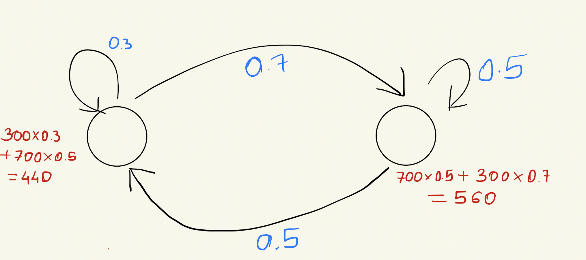
Let’s start by looking at a simple Markov process involving two states: Happy and Stressed.
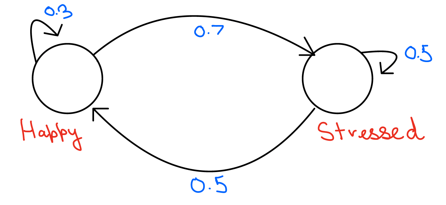
In the figure above, we have two states: Happy and Stressed.
Here’s what we know:
- 70% of people in the Happy state will become Stressed after some time (one iteration), while 30% will stay Happy.
- 50% of people in the Stressed state will become Happy after some time (one iteration), while 50% will stay Stressed.
Now, consider an initial scenario where there are 1000 people in the Happy state and 0 in the Stressed state. What will the distribution of people be after several iterations? Will it remain the same?
Let’s try to do this for two iterations:
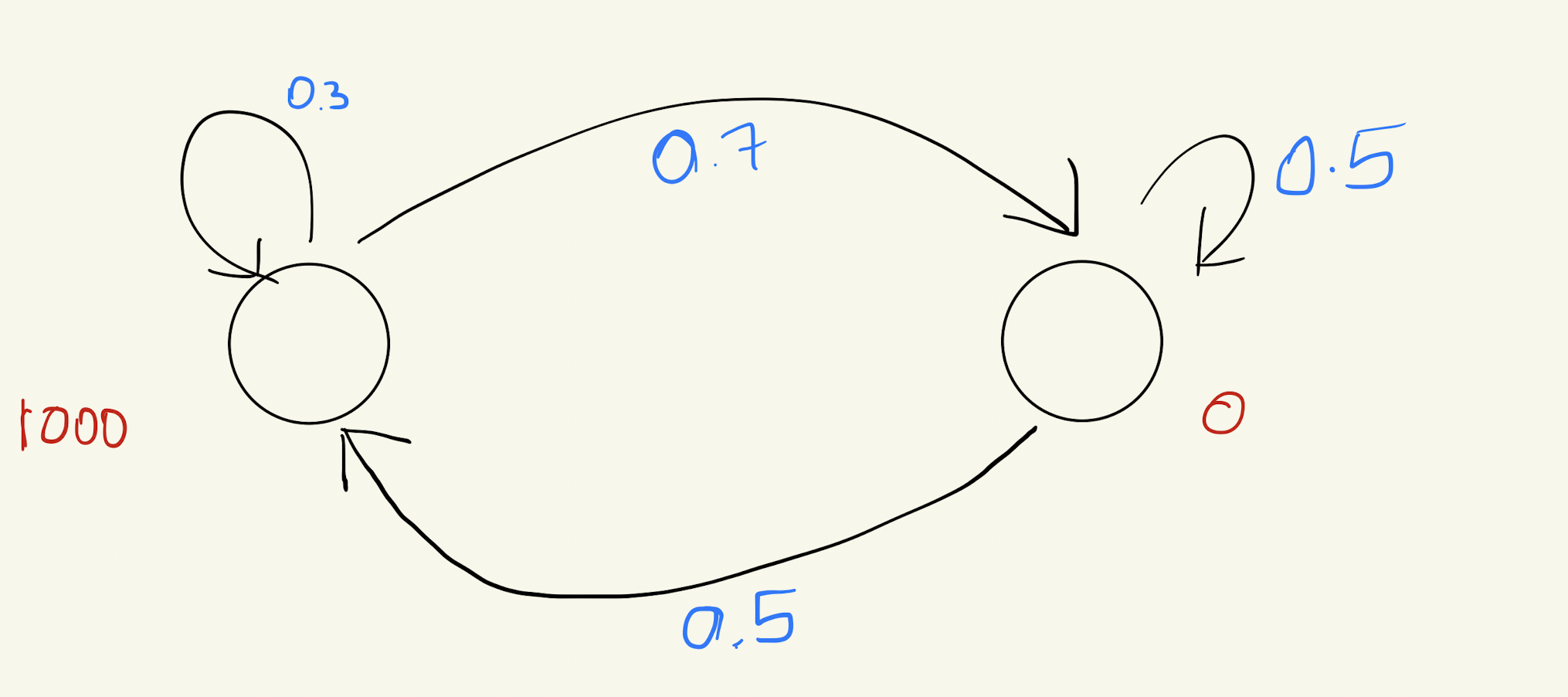
Do you notice how the distribution changes after two iterations?
Will it keep changing, or will it eventually stabilize?
Yes, it will converge after some time. But do you understand why?
To get a better understanding, you can write a program to see if this distribution converges over time. Here’s a simple code snippet to help you explore this:
import numpy as np
A = np.array([[0.3, 0.5],[0.7, 0.5]]) # Transition matrix
v = np.array([1000, 0]) # Initial distribution
def iterate_until_convergence(A, v, tolerance=1e-6, max_iterations=10):
    for _ in range(max_iterations):
        v_next = A @ v
        if np.allclose(v, v_next, atol=tolerance):
            return v_next
        v = v_next
    return v
final_distribution = iterate_until_convergence(A, v)
total_population = np.sum(final_distribution)
percentage_distribution = final_distribution / total_population * 100
print(final_distribution, percentage_distribution)
Notice how the distribution changes with each iteration. Eventually, you’ll see that it stops changing—it converges.
Matrix Method
There’s another way to approach this: through matrix operations.
Think of the probability of transitioning from one state to another as a matrix, and the initial distribution of people in both states as a vector.
Here’s what the matrix looks like:
\[\text{Transition Matrix: } M = \begin{pmatrix} 0.7 & 0.5 \\ 0.3 & 0.5 \end{pmatrix}\]Notice that the sum of the columns is 1.
And here’s the initial distribution vector:
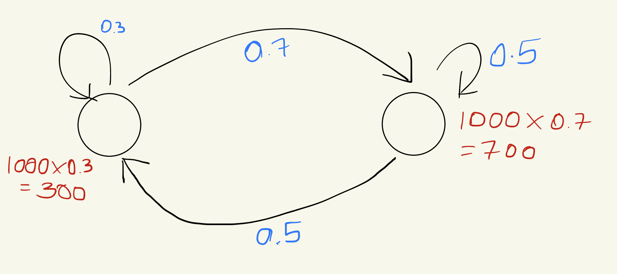
\[\text{Initial Vector: } v_0= \begin{pmatrix} 1000 \\ 0 \end{pmatrix}\]Now, to predict the distribution after one iteration, you multiply the matrix with the vector:
\[\text{New Distribution: } v_1 = \begin{pmatrix} 0.7 & 0.5 \\ 0.3 & 0.5 \end{pmatrix} \begin{pmatrix} 1000 \\ 0 \end{pmatrix} = \begin{pmatrix} 700 \\ 300 \end{pmatrix}\]So, to find the eventual distribution, would you keep performing matrix multiplications repeatedly?
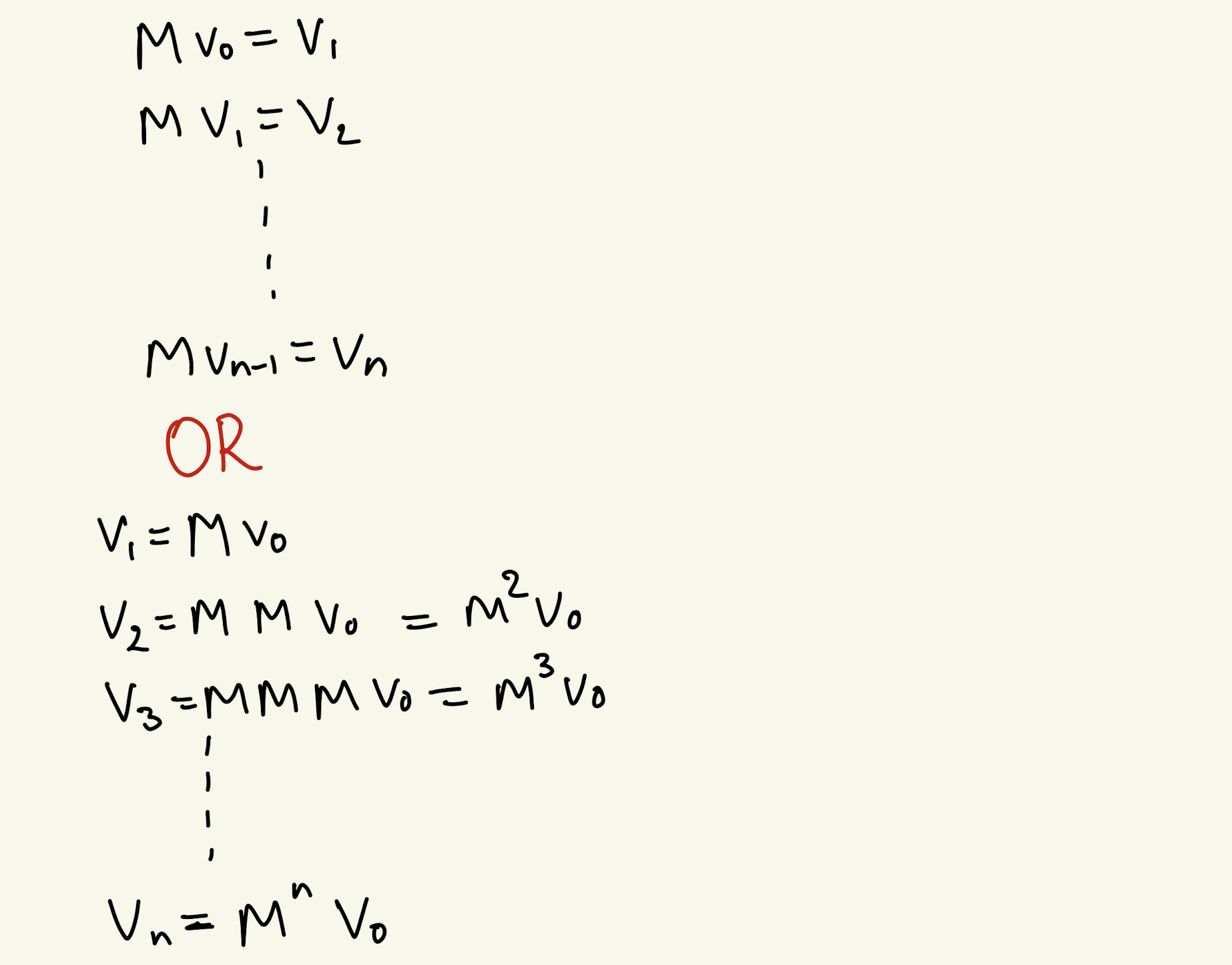
But do you realize that you don’t need to do the matrix multiplication all the time? You just need to find \(M^{n}\).
But \(M\) is a matrix, so how easily can you compute \(M^{n}\)?
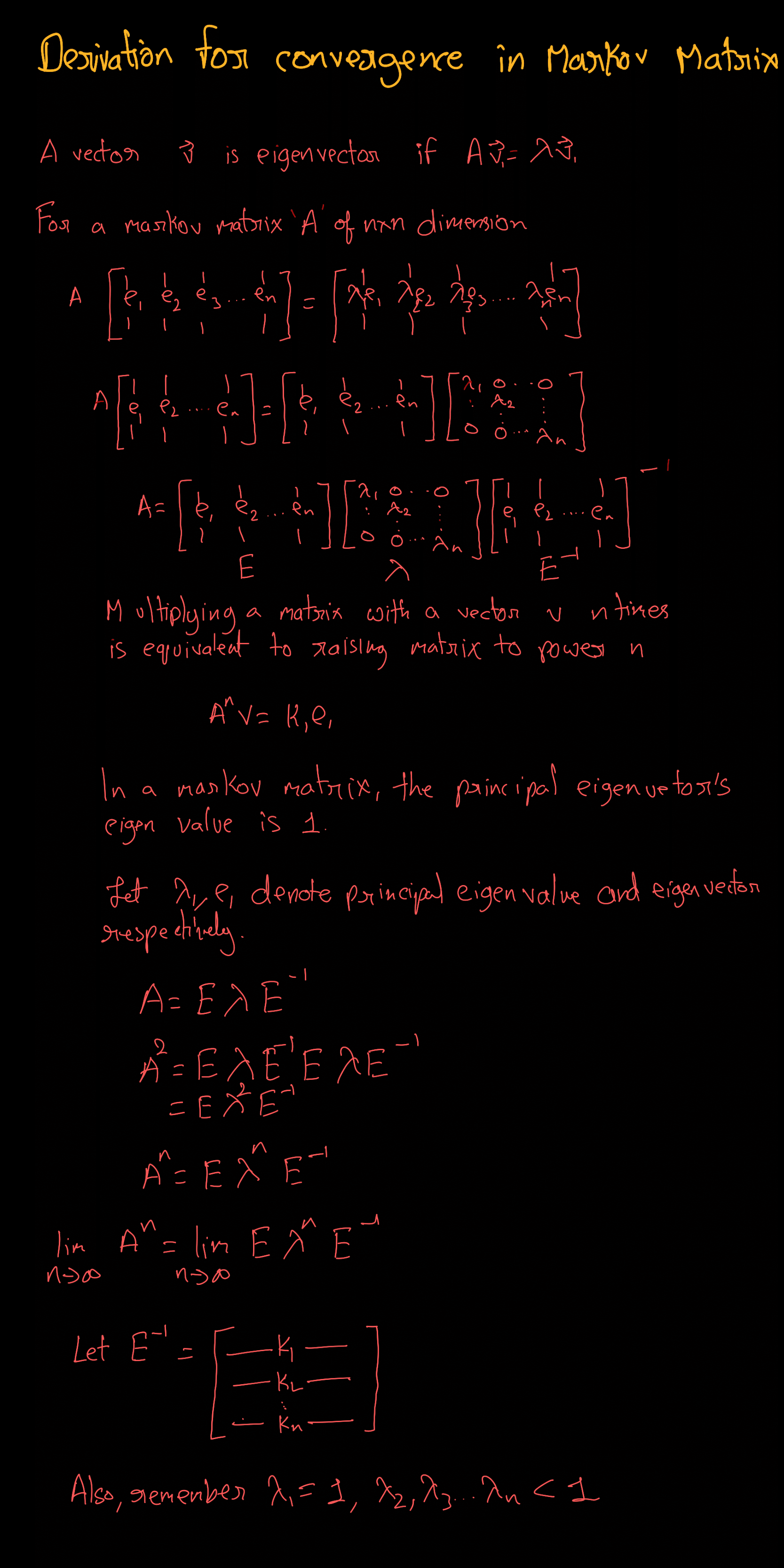
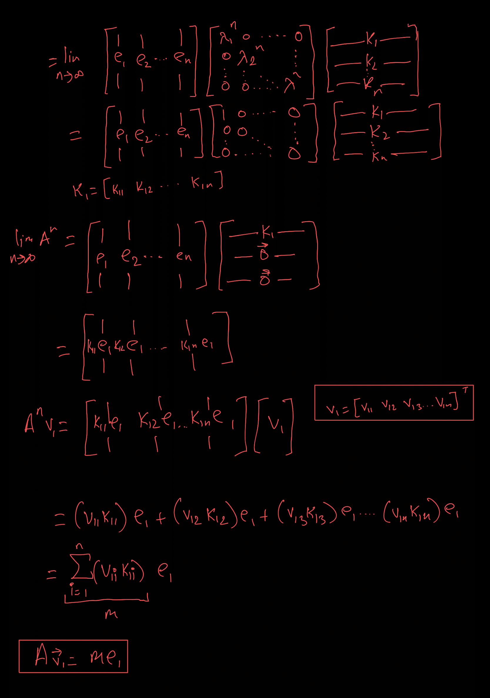
This is where EVD (Eigenvalue Decomposition) comes to our rescue!
EVD, or Eigenvalue Decomposition, allows us to express the matrix \(M\) in terms of its eigenvalues and eigenvectors.
We know that:
\[A v = \lambda v\]where \(v\) is the eigenvector and \(\lambda\) is the corresponding eigenvalue.
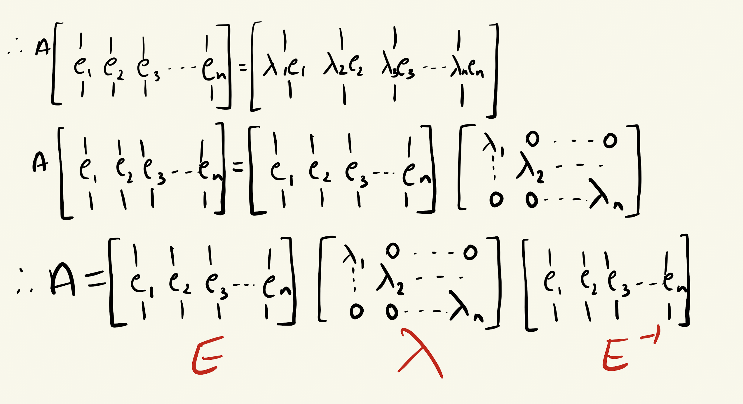
Multiplying a matrix by a vector \(v\) \(n\) times is equivalent to raising the matrix to the power \(n\).
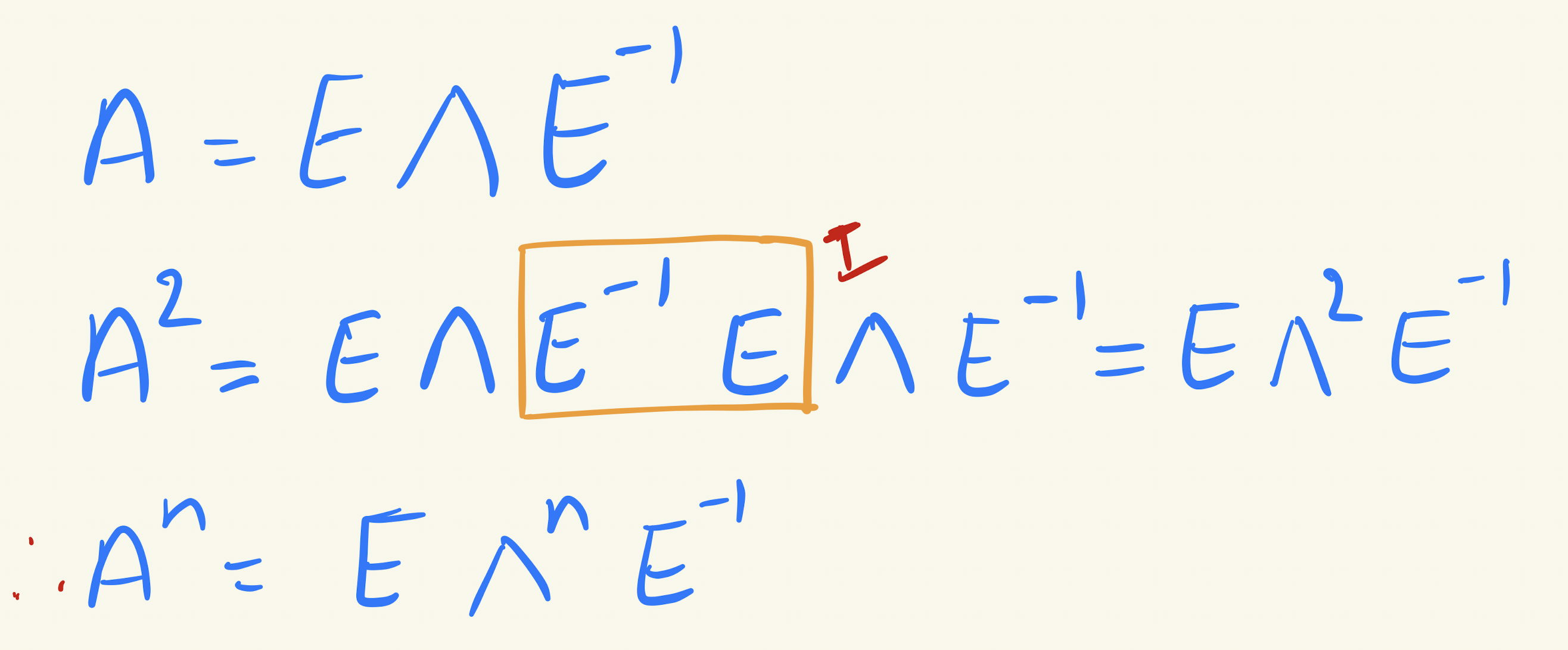
Now, do you realize the importance and power of eigenvectors? They can be used to find any power of \(A\) in no time.
Over time, this matrix multiplication will lead to a steady-state distribution, where further iterations will not change the result. This is the point of convergence.
So for the above example, we get the final distribution to be:
\[\begin{bmatrix} 416.666368 \\ 583.333632 \end{bmatrix}\]Derivation for convergence in Markov Matrix
 Credits: Aditya BMV
Application of Markov Matrices: Opening a New Restaurant
Imagine you want to start a new restaurant in the city. Where should you situate it? Near the railway station? Near the IT hub? Near schools?
The best way to determine the ideal location is by using the Markov matrix technique. Here’s the idea:
By analyzing the movement of people throughout the day, you can figure out where the maximum number of people eventually gather. This will be the hotspot for your restaurant.
Using a Markov matrix, you can model the probabilities of people moving from one location to another over time. As you apply the matrix iteratively, you’ll see that the distribution of people converges to a steady state.
The location with the highest steady-state probability is where people are most likely to gather, making it the best spot for your restaurant. This method allows you to make a data-driven decision, increasing the chances of your restaurant’s success.
Taylor Series
Question: Can You Find a Polynomial Function That Maps a Set of Inputs to Outputs?
Given a set of input and output values, how can we find a polynomial function that accurately maps those inputs to the corresponding outputs? This is a common problem in mathematics and data modeling, where we try to fit a curve to data points.
Example: Suppose we are given the following set of input and output pairs:
| \(x\) | \(f(x)\) |
|---|---|
| 1 | 2 |
| 2 | 3 |
| 3 | 12 |
| 4 | 35 |
Our goal is to find a polynomial \(p(x) = a_nx^n + a_{n-1}x^{n-1} + \cdots + a_1x + a_0\) that satisfies these input-output relations.
Step-by-Step Approach (First Principles):
-
Assume a polynomial form: Start by assuming the simplest polynomial that could fit these points. For four data points, we may try a cubic polynomial: \(p(x) = ax^3 + bx^2 + cx + d\)
-
Set up equations: Substitute the given points into this polynomial.
- For \(x = 1\), \(f(1) = 2\): \(a(1)^3 + b(1)^2 + c(1) + d = 2 \Rightarrow a + b + c + d = 2\)
- For \(x = 2\), \(f(2) = 3\): \(a(2)^3 + b(2)^2 + c(2) + d = 3 \Rightarrow 8a + 4b + 2c + d = 3\)
- For \(x = 3\), \(f(3) = 10\): \(a(3)^3 + b(3)^2 + c(3) + d = 10 \Rightarrow 27a + 9b + 3c + d = 12\)
- For \(x = 4\), \(f(4) = 27\): \(a(4)^3 + b(4)^2 + c(4) + d = 27 \Rightarrow 64a + 16b + 4c + d = 35\)
-
Solve the system of equations: Now, solve this system of four linear equations for \(a\), \(b\), \(c\), and \(d\).
Solving these, we get: \(a = 1, \quad b = -2, \quad c = 0, \quad d = 3\)
-
Write the polynomial: The polynomial function that maps the inputs to the outputs is: \(p(x) = x^3 - 2x^2 + 3\)
Polynomial Approximation for Complex Functions
Now that we’ve seen how to derive a polynomial that fits specific points, let’s consider more complex functions like \(\sin(x)\), \(\cos(x)\), and \(e^x\), which can’t be exactly represented by simple polynomials. However, using a powerful mathematical tool called the Taylor series, we can approximate these functions very closely using polynomials.
Taylor Series: Approximating Functions with Polynomials
The Taylor series allows us to approximate functions that are smooth (infinitely differentiable) with polynomials. The key idea is to express a function as an infinite sum of terms derived from the function’s derivatives at a specific point.
What Does the Taylor Series Depend On?
The accuracy of the Taylor series approximation depends on two main factors:
- The differentiability of the function: The function must be differentiable as many times as needed at the point around which the approximation is made.
- The number of terms: More terms in the series result in a better approximation.
The Taylor Series Formula: Given a function \(f(x)\), its Taylor series expansion around \(x = a\) is given by:
\[f(x) = f(a) + f'(a)(x - a) + \frac{f''(a)}{2!}(x - a)^2 + \frac{f^{(3)}(a)}{3!}(x - a)^3 + \cdots\]For most practical purposes, we truncate the series after a few terms to get an approximate polynomial.
Example: Taylor Series for Common Functions
-
Exponential Function \(e^x\): \(e^x = 1 + x + \frac{x^2}{2!} + \frac{x^3}{3!} + \cdots\) This series is valid for all \(x\), and the more terms you include, the more accurate the approximation.
-
Sine Function \(\sin(x)\): \(\sin(x) = x - \frac{x^3}{3!} + \frac{x^5}{5!} - \frac{x^7}{7!} + \cdots\) The sine function is odd, so all even powers of \(x\) vanish.
-
Cosine Function \(\cos(x)\): \(\cos(x) = 1 - \frac{x^2}{2!} + \frac{x^4}{4!} - \frac{x^6}{6!} + \cdots\) The cosine function is even, so all odd powers of \(x\) vanish.
Taylor Series and Function Behavior
By approximating complex functions using polynomials derived from the Taylor series, we can understand how functions behave near a particular point. For instance, for small values of \(x\), the sine function behaves almost linearly, as the higher-order terms contribute very little.
Summary:
The Taylor series allows us to approximate complex, real-world functions using simpler polynomials, similar to how machine learning models aim to approximate the underlying patterns in data. Both involve the concept of approximation and rely on increasing complexity (more terms in the series or more features in the model) to improve accuracy.
Gradient Descent
Introduction
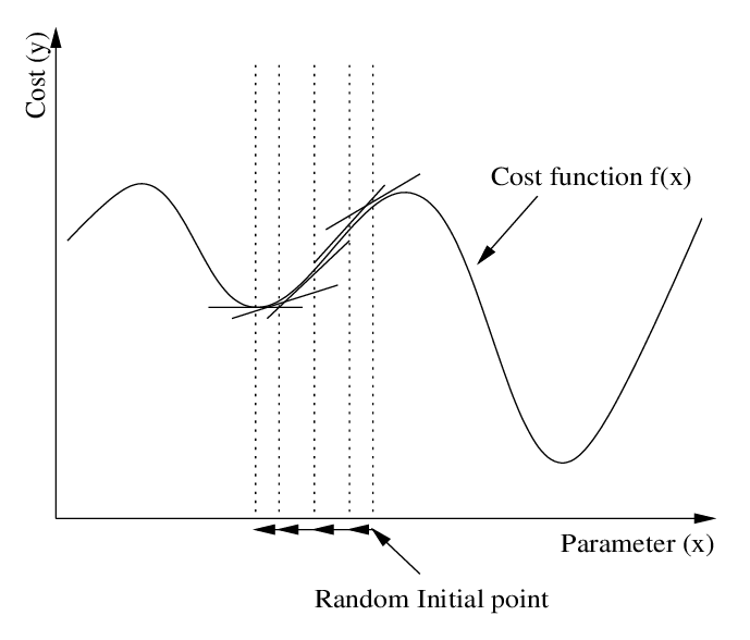
Gradient Descent is an optimization algorithm that helps us find the minimum value of a function by iteratively moving in the direction of the steepest descent. You can think of it as a way to slide down a hill to reach the lowest point, starting from any point on the hill.
What is Gradient Descent?
Imagine you are standing on a hill, and your goal is to reach the bottom, but it’s dark, and you can’t see anything. The only thing you can sense is the slope of the ground beneath your feet.
- Steepest Descent: Each step you take is in the direction that feels the steepest downward.
- Learning Rate: The size of each step you take is controlled by how confident you feel. If you take very large steps (high learning rate), you might overshoot the bottom, but if you take very small steps (low learning rate), you’ll reach the bottom slowly.
This is essentially how Gradient Descent works! It “feels” the slope of the function you’re trying to minimize (called the gradient) and takes steps in the steepest downward direction to find the minimum.
Intuitive Examples
Example 1: A Simple Hill
Let’s take a simple example: imagine you’re skiing down a smooth, bowl-shaped hill. The objective is to get to the lowest point. At every moment, you assess which direction takes you down most steeply. You take small steps in that direction, each time reassessing the steepest descent until you finally arrive at the bottom.
Mathematically, if the hill is represented by the function \(J(\Theta) = (\Theta - 3)^2\), Gradient Descent will start at some point on the curve and iteratively move towards the minimum point at \(\Theta = 3\).
Example 2: Finding the Minimum of a Valley
Now, think of Gradient Descent as navigating a deep valley. You start at some random point on one of the slopes and use the slope of the valley to guide you downwards.
- Steeper Slope: If you’re at a steep section of the valley, you know to take bigger steps.
- Flatter Slope: If the slope gets shallower, you take smaller steps because you’re nearing the bottom.
Key Insight: The steeper the slope (larger gradient), the bigger the step you take; the flatter the slope (smaller gradient), the smaller the step. This way, you don’t overshoot the minimum.
Example 3: Rolling a Ball Down a Hill
Another analogy is to think of rolling a ball down a hill. If the hill is steep, the ball accelerates fast. As the ball gets closer to the bottom where the slope is gentler, it slows down and finally comes to a stop at the lowest point.
In terms of Gradient Descent:
- The gradient is like the steepness of the hill, determining how fast the ball will roll.
- The learning rate is how much we allow the ball to roll at each step.
Given a convex function \(J(Θ)\),
Gradient Descent follows the update rule: \(\Theta^{(t+1)} = \Theta{(t)} − \eta \nabla_{\Theta} J(\Theta^{(t)})\)
How Does Gradient Descent Work?
Let’s break it down into steps:
- Start at a Random Point: Imagine being placed randomly on a hill. This is like starting Gradient Descent at an initial guess for the parameter \(\Theta\).
- Compute the Slope (Gradient): At each point, you calculate the slope of the hill, which tells you in which direction the function increases or decreases most rapidly.
- Take a Step in the Opposite Direction: You take a step in the direction opposite to the gradient (i.e., you move downwards). The size of this step is determined by the learning rate \(\eta\).
- Repeat: You keep taking steps until you reach the bottom, i.e., until the slope becomes nearly zero (the gradient becomes very small).
Visualizing Gradient Descent
Graphical Representation in 1D
Imagine we have a curve representing a simple function, say \(J(\Theta) = (\Theta - 3)^2\), which looks like a bowl. If you start at some point on the curve, Gradient Descent will move you step-by-step towards the minimum.
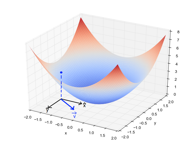
Graphical Representation in Multiple Dimensions
In higher dimensions, Gradient Descent works similarly. Instead of a curve, think of a hilly landscape. You can start at any point in this landscape, and Gradient Descent will help you find the lowest point in this multidimensional terrain.
Here is an example of how Gradient Descent works in a 3D valley, where the algorithm gradually moves towards the minimum:
Variants of Gradient Descent
There are a few popular variants of Gradient Descent that improve efficiency, especially for large datasets:
- Batch Gradient Descent: Uses all data points to compute the gradient in each step.
- Stochastic Gradient Descent (SGD): Uses a single data point at a time to update the parameters. It can move faster but introduces some noise into the updates.
- Mini-Batch Gradient Descent: A compromise between batch and stochastic, where a small group of data points (mini-batch) is used to update the parameters.
Conclusion
Gradient Descent is a powerful yet intuitive method to find the minimum of a function. By constantly moving in the direction of steepest descent (downhill), we eventually find the lowest point. Whether it’s finding the best fit line in linear regression, training deep neural networks, or solving any optimization problem, Gradient Descent is a fundamental tool in machine learning.
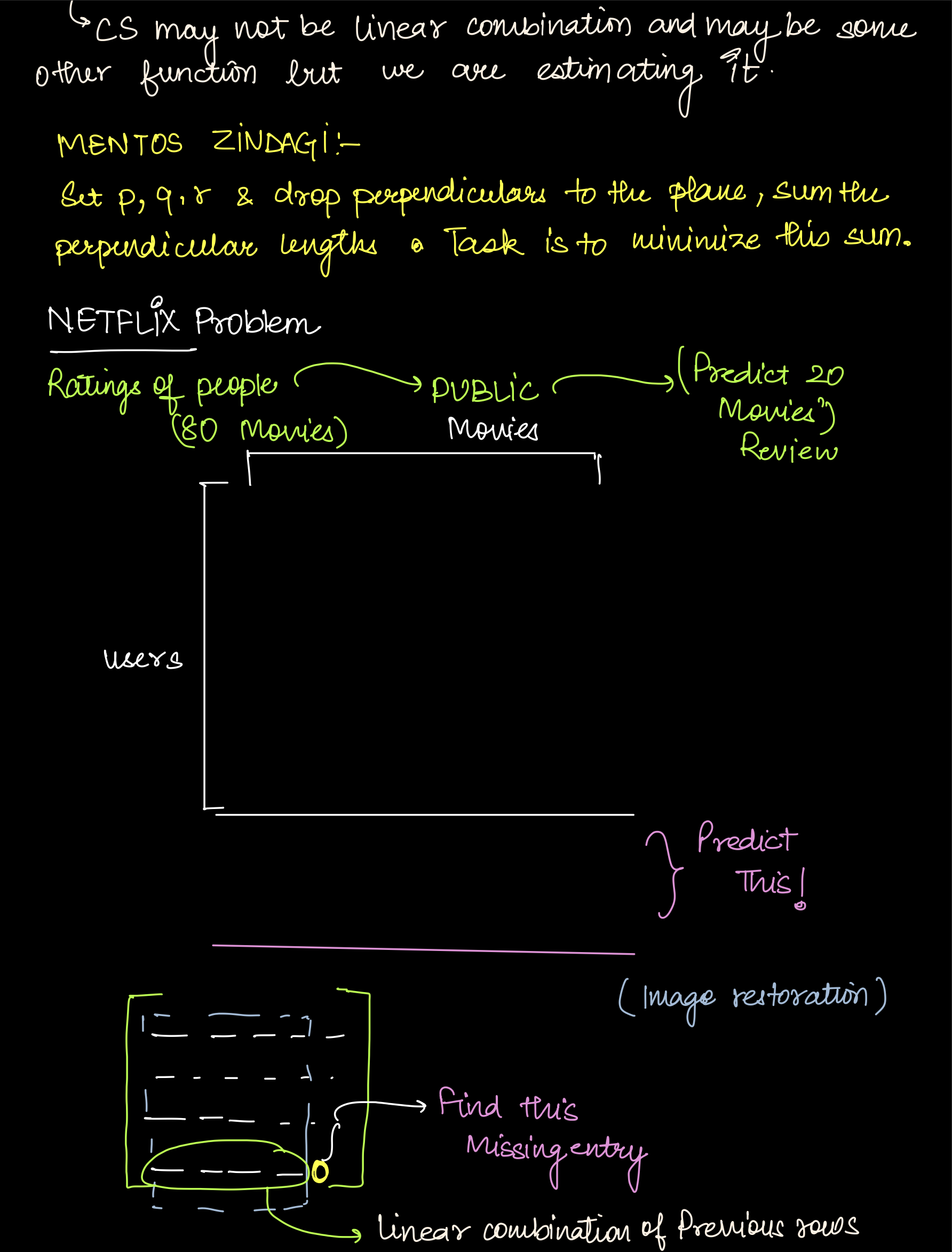
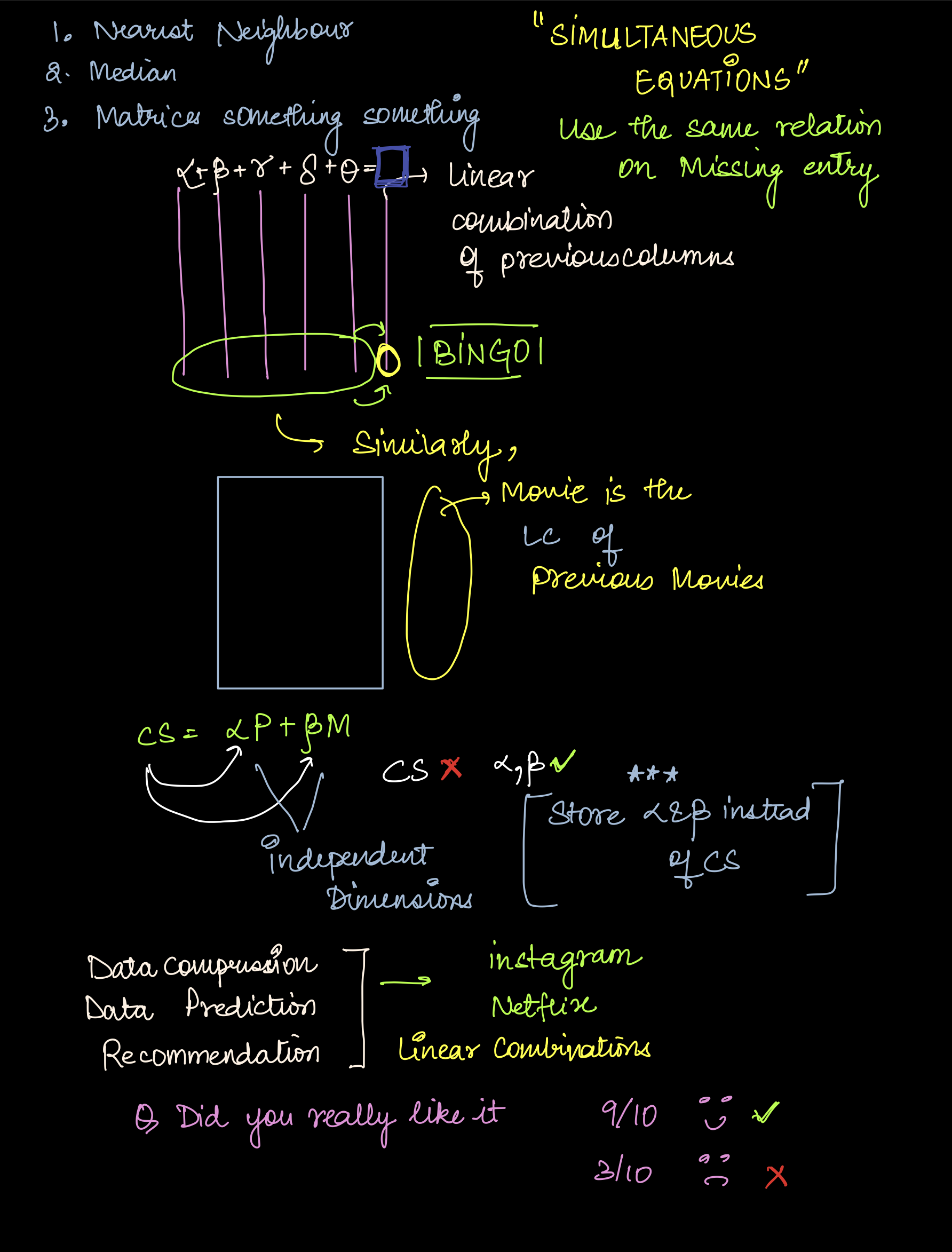
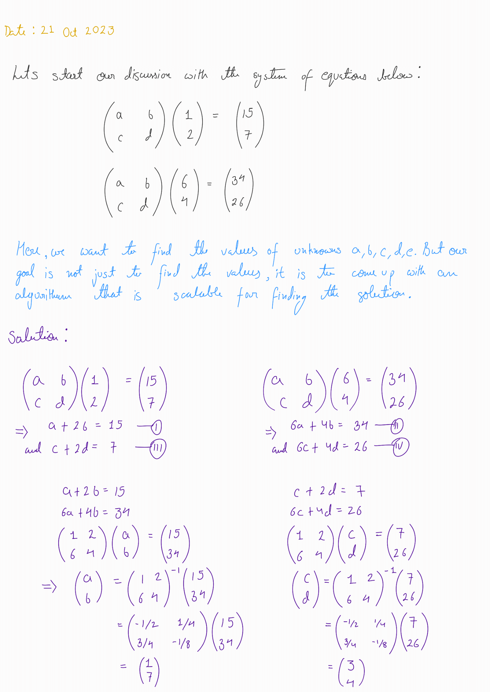
Least Squares
Subjects Example
Let’s dive into an interesting question: What does it mean to take points in 3D and project them onto a 2D plane? Imagine you have a table with marks in Physics, Math, and Programming.
\[\text{Programming} = \alpha \cdot \text{Physics} + \beta \cdot \text{Math} + \text{Some noise}\]Now, if you’re given the marks in Physics, Math, and Programming, can you plot them on a plane? What would that look like?
Observe the following table:
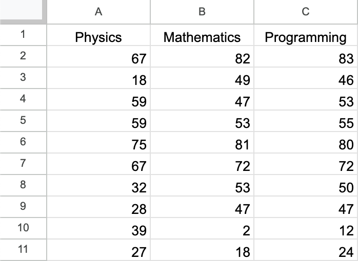
Take a look at this plot. You’ll notice that not all the points lie perfectly on the plane, but they are very close to it. This suggests that we can approximate these points using this plane.
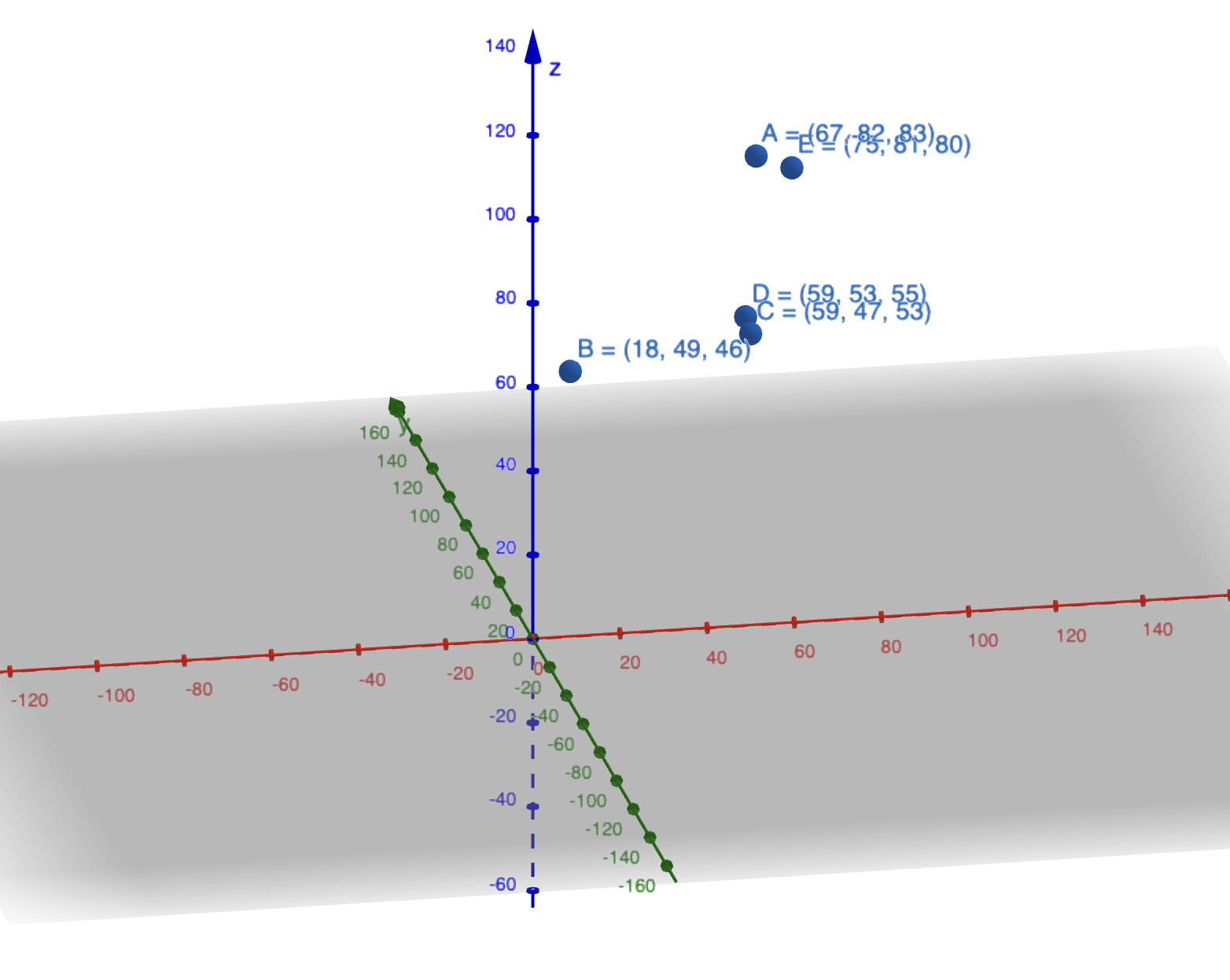
But how do we find the best possible plane? Well, to do that, we need to minimize the distance of the points from the plane.
Can you think of how we might achieve that? How would you go about finding the plane that best fits the data?
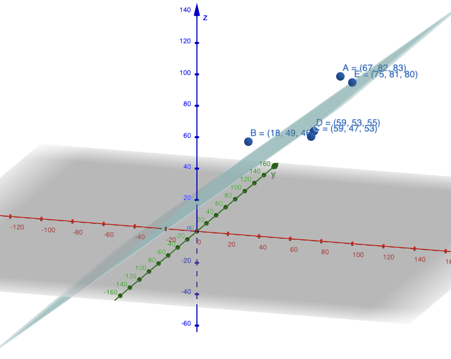
Projection of Points
Now, let’s shift our focus to the concept of projection. Observe the following graph: some points lie on or close to a plane.
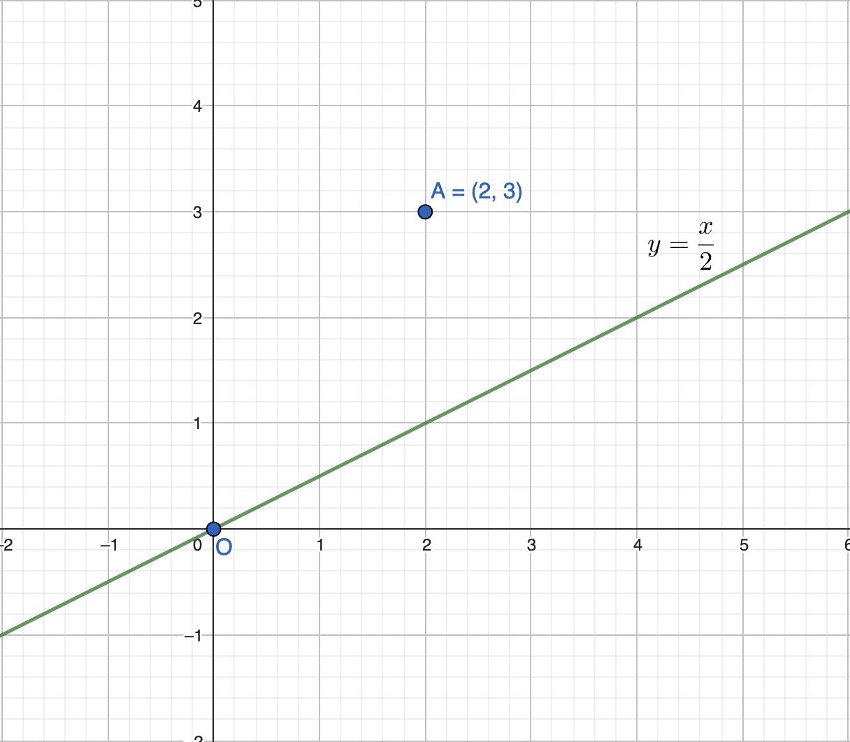
But what if we want to find the shortest distance of a specific point, say point A, from a given line like \(y = \frac{x}{2}\)? How would you do that?
The answer is simple: it’s the perpendicular drop from point A onto the line.
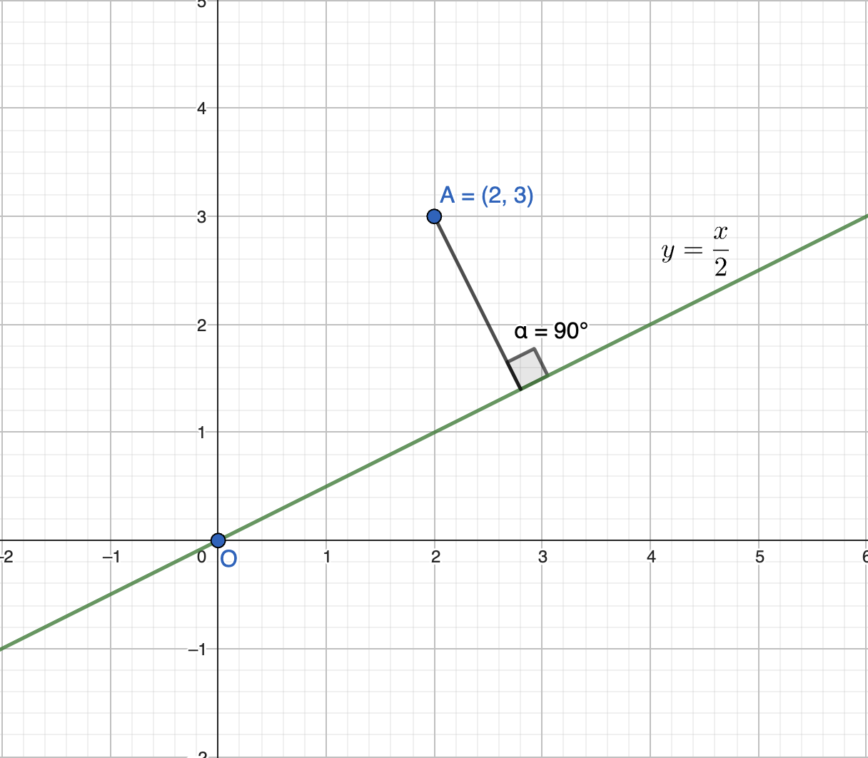
This is known as the projection of vector \(p\) onto the line \(y = \frac{x}{2}\).
But how can you figure out a generic method for finding this projection?
The dot product offers a straightforward approach. Consider a point \(v\) on this line and take the dot product of \(v\) with \(p\). For instance, if \(v = (1, 2)\), the dot product gives us the necessary information to determine the projection.
Would you like to see the math behind it? Here’s how it works:
\[v \cdot (\alpha v - b) = 0\] \[\alpha \cdot v^T v = v^T b\] \[\alpha = \frac{v^T b}{v^T v}\]Substituting the values:
\[\alpha = \frac{\begin{bmatrix} 2 & 1 \end{bmatrix} \begin{bmatrix} 2 \\ 3 \end{bmatrix}}{\begin{bmatrix} 2 & 1 \end{bmatrix} \begin{bmatrix} 2 \\ 1 \end{bmatrix}} = \frac{7}{5} = 1.4\]So, the projection of point A onto the line \(y\) is given by:
\[B = (\alpha \cdot 2, \alpha \cdot 1) = (2.8, 1.4)\]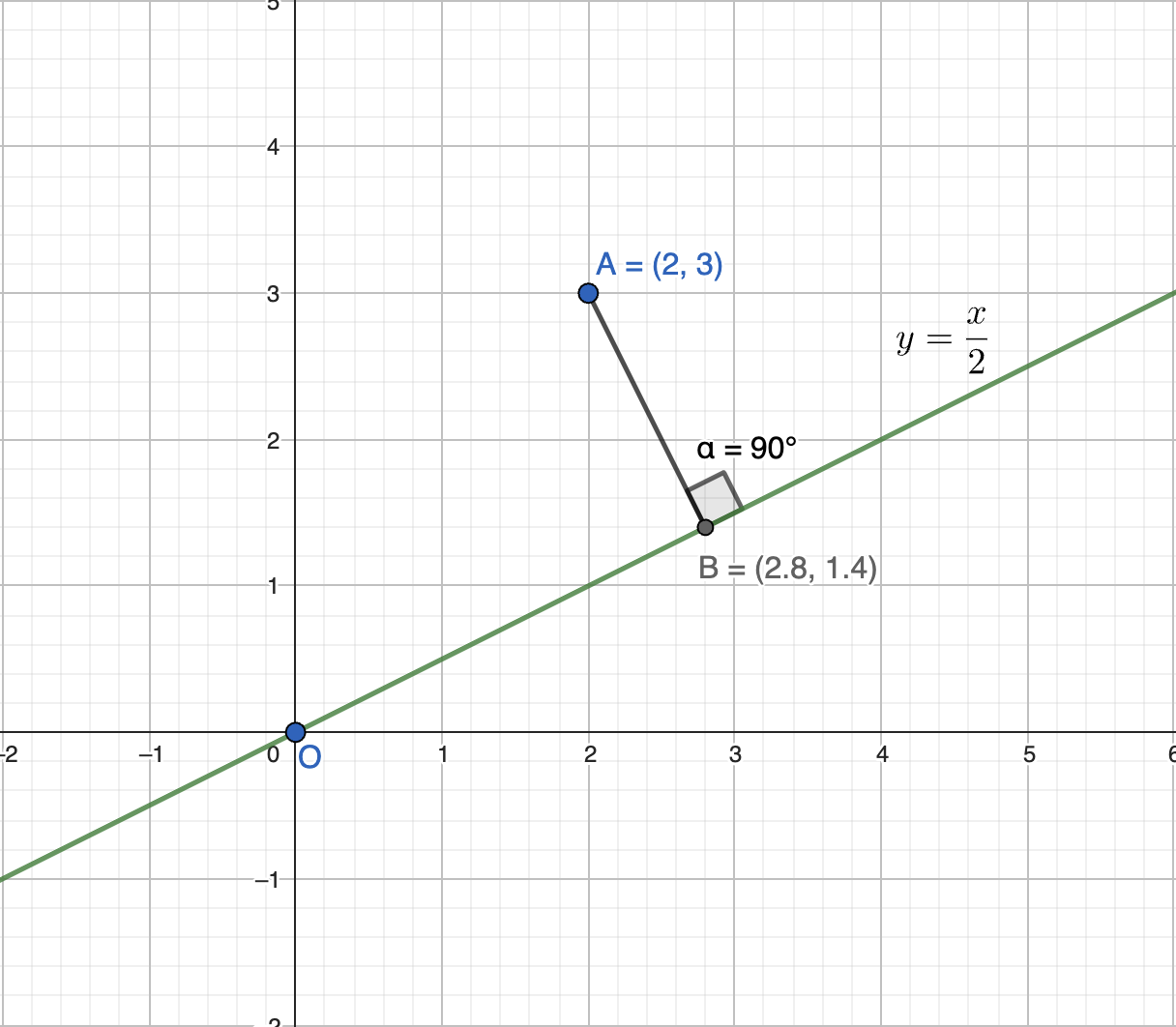
This is a simple yet powerful method. But there’s more to it.
Let’s think about matrices. What if we take this concept further? Consider the equation:
\[A(A \cdot \bar{x} - b) = 0\]To solve for \(\bar{x}\), we rearrange it as:
\[A^T A \bar{x} = A^T b\] \[\bar{x} = (A^T A)^{-1} A^T b\]And then:
\[A \bar{x} = A(A^T A)^{-1} A^T b\]You see how everything falls into place, right? But here’s a critical point: this works perfectly if ( A ) is invertible. Now, think about the real world—most matrices are invertible, aren’t they? So, we don’t usually have to worry about invertibility here. But what would happen if a matrix wasn’t invertible? How would that affect our calculations?
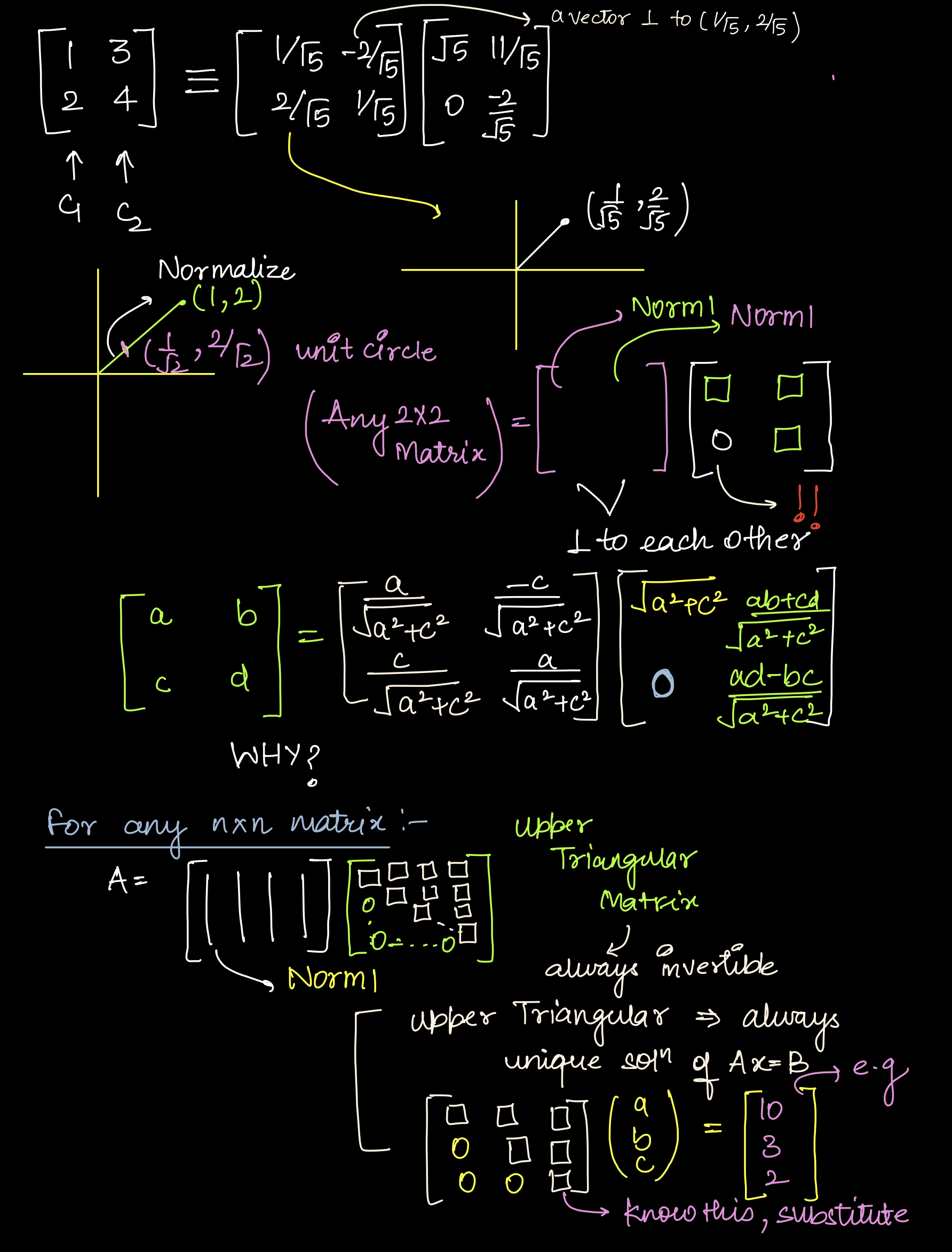
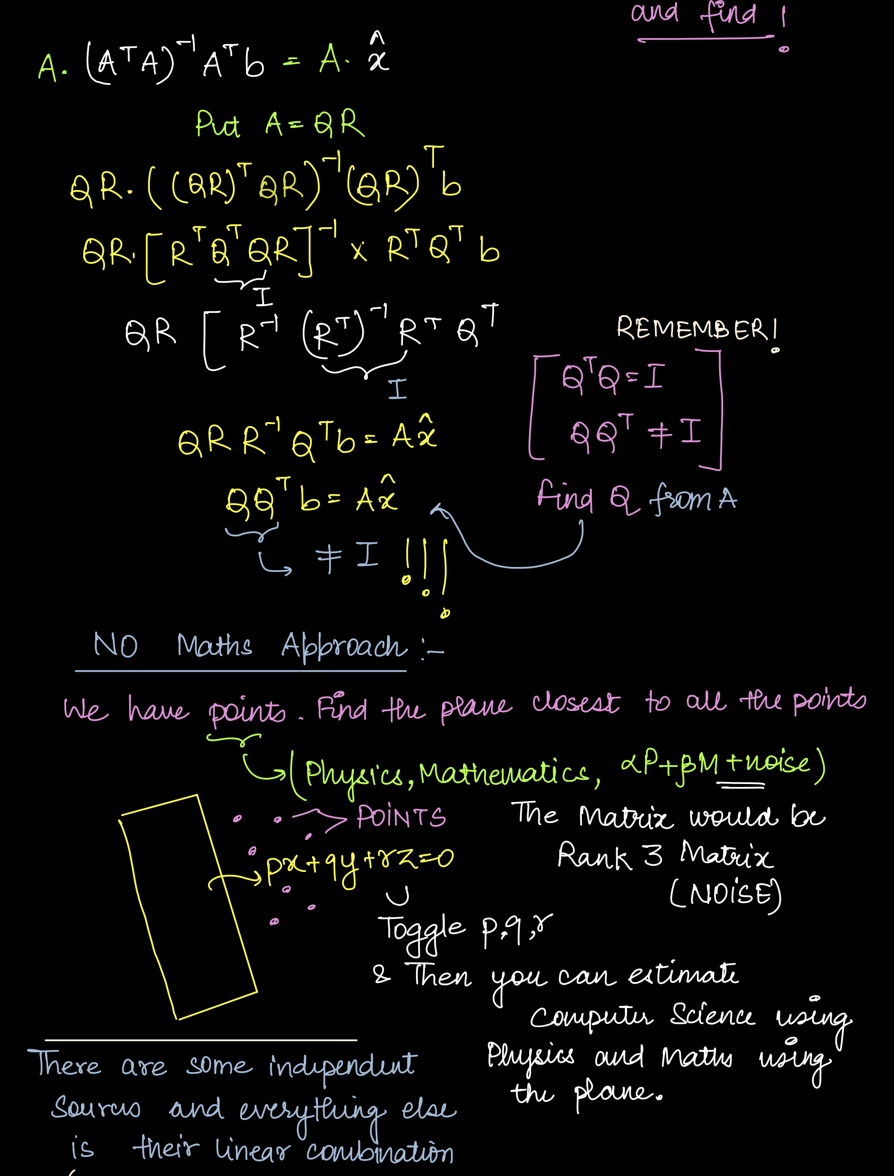
QR Factorization
Credits: Lakshay
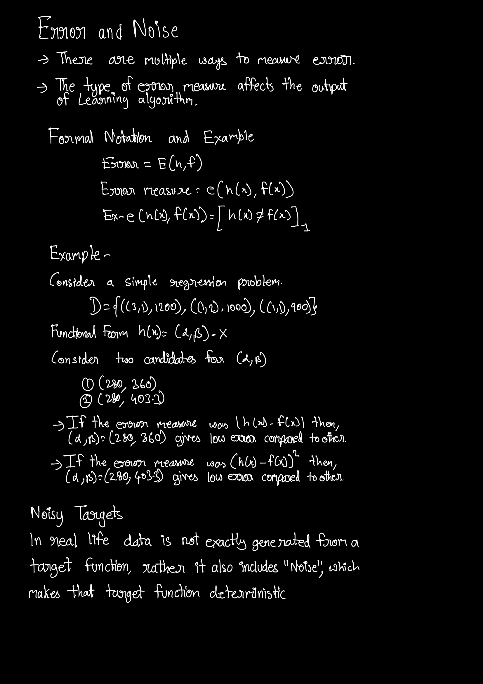
Hoeffding’s inequality
Question: Walk into Amritsar and estimate the ratio of men to women for a population of \(10^6\). Write a code and observe this.
# create a list of length L of 1 million of randomly distributed numbers between one and zero with probability 0.21

import random

l = 10000
result = [0 if random.random() < 0.21 else 1 for _ in range(l)]
print(result)
#create another list with ith entry being the proportion of 0s seen so far, meaning, upto the ith position in the original list
# this can be done by using the cumulative sum of the original list, and then dividing by the index

result3 = [sum(result[:i])/i if i != 0 else 0 for i in range(1, l)]
print(result3)
# create_list(p_zero, n): "Generate a Python function in Colab to create a list of length n where each element is either 0 or 1, with a given probability p_zero for zeros."
def create_list(p_zero, n):
    import random
    return [random.choices([0, 1], weights=[p_zero, 1-p_zero])[0] for _ in range(n)]
# cumulative_proportion_ones(L): "Create a Python function in Colab that takes a list of 0s and 1s and returns the cumulative proportion of 1s at each position."
def cumulative_proportion_ones(L):
    return [sum(L[:i+1])/(i+1) for i in range(len(L))]

# create parameters p_zero, n, n_small, window_size
p_zero = 0.21
n = 10000
n_small = 10
window_size = 5

#Plotting Cumulative Proportion: "Write Python code in Colab to plot the cumulative proportion of 1s from a list generated with a specific zero probability using Matplotlib."
import matplotlib.pyplot as plt
L = create_list(p_zero, n)
plt.plot(cumulative_proportion_ones(L))
plt.show()

# Error Calculation: "Generate Python code in Colab to calculate and plot the error between the cumulative proportion of 1s and the expected value over time."
# Calculate errors
errors = [abs(prop - (1-p_zero)) for prop in cumulative_proportion_ones(L)]

# Plot errors
plt.plot(errors)
plt.xlabel('Time')
plt.ylabel('Error')
plt.title('Error between Cumulative Proportion of 1s and Expected Value')
plt.show()
You have a biased coin. How or when will you get to know that the coin is biased, or how many steps will it take to know that the coin is biased?
It is given by:
\[Pr(|\mu - \gamma| > \epsilon) \leq \frac{2}{e^{2 \epsilon^{2} N}}\]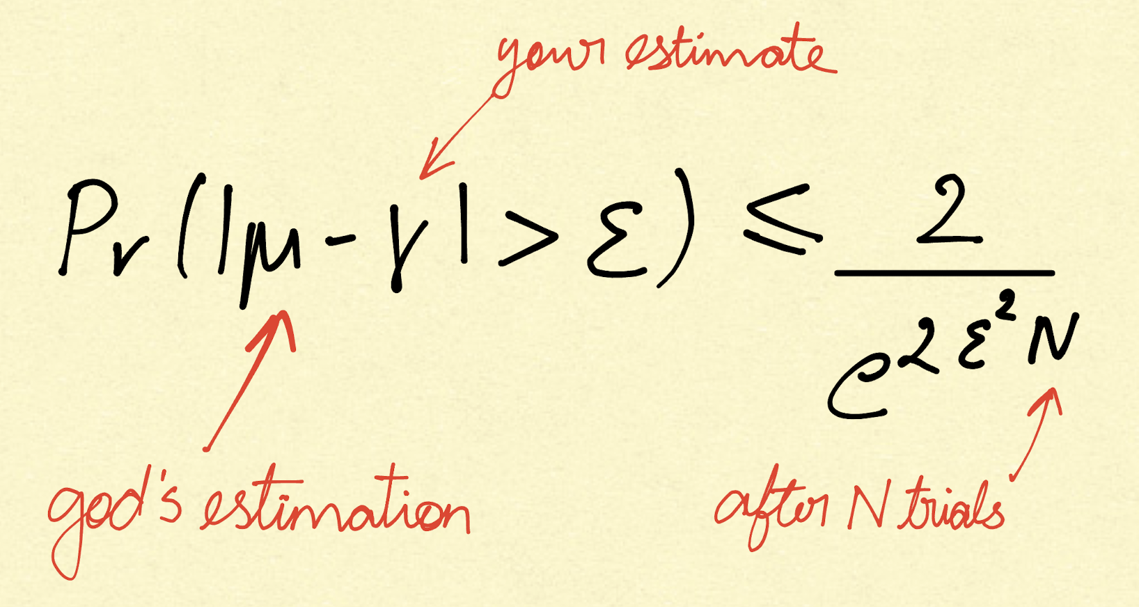
Here, \(\epsilon\) can be anything like 0.001 or 0.01, but on the right-hand side, \(\epsilon\) is squared:
\[\epsilon^2 \to 0\]This makes it very small, pulling the denominator of the right-hand side closer to 1, as you might expect! But N (the number of samples) pulls it up.
So, the chances of the difference between the true mean and your estimated mean being greater than \(\epsilon\) are:
\[\leq \frac{1}{e^{2 \epsilon^{2} N}}\]How do we apply this logic to our question?
You can see that with a very small N, convergence occurs quickly. Do you realize that the whole of this process is dependent on N and that there is an exponential dip?
Hoeffding’s Inequality and its Relation with N
import random
import matplotlib.pyplot as plt
import time

def create_list(p_zero, n):
    L = []
    for _ in range(n):
        if random.random() < p_zero:
            L.append(0)  # Probability p_zero of appending 0
        else:
            L.append(1)  # Probability 1 - p_zero of appending 1
    return L

def cumulative_proportion_ones(L):
    cumulative_proportion = []
    cumulative_sum = 0
    for i in range(len(L)):
        cumulative_sum += L[i]
        cumulative_proportion.append(cumulative_sum / (i + 1))
        # print(f"Progress: {i}, {cumulative_sum/(i+1)}")
    return cumulative_proportion

# Parameters
p_zero = 0.21  # Probability of 0
n = 100000   # Length of the list for full plot
n_small = 100000 # Length of the list for error calculation
window_size = 10  # Number of errors to include in each average calculation

# Create the list
L = create_list(p_zero, n)

# Calculate the cumulative proportion of 1's
cumulative_ones = cumulative_proportion_ones(L)

# Plot the cumulative proportion of 1's over time
plt.figure(figsize=(12, 6))
plt.subplot(1, 2, 1)
plt.plot(cumulative_ones, label=f'Proportion of 1s (p_zero = {p_zero})')
plt.axhline(y=1 - p_zero, color='r', linestyle='--', label='Expected Proportion of 1s')
plt.xlabel('Number of Elements')
plt.ylabel('Cumulative Proportion of 1s')
plt.title('Cumulative Proportion of 1s Over Time')
plt.legend()

# Smaller list for error calculation
L_small = create_list(p_zero, n_small)

# Calculate the cumulative proportion of 1's
cumulative_ones_small = cumulative_proportion_ones(L_small)

# Expected proportion of 1's
expected_proportion = 1 - p_zero

# Calculate the error between the cumulative proportion and the expected proportion
error = [abs(cumulative_ones_small[i] - expected_proportion) for i in range(n_small)]

# Plot the error over time
plt.subplot(1, 2, 2)
plt.plot(error, label='Error between Cumulative Proportion and Expected Proportion', color='orange')
plt.xlabel('Number of Elements')
plt.ylabel('Error')
plt.title('Error Between Cumulative Proportion of 1s and Expected Value')
plt.legend()
plt.show()
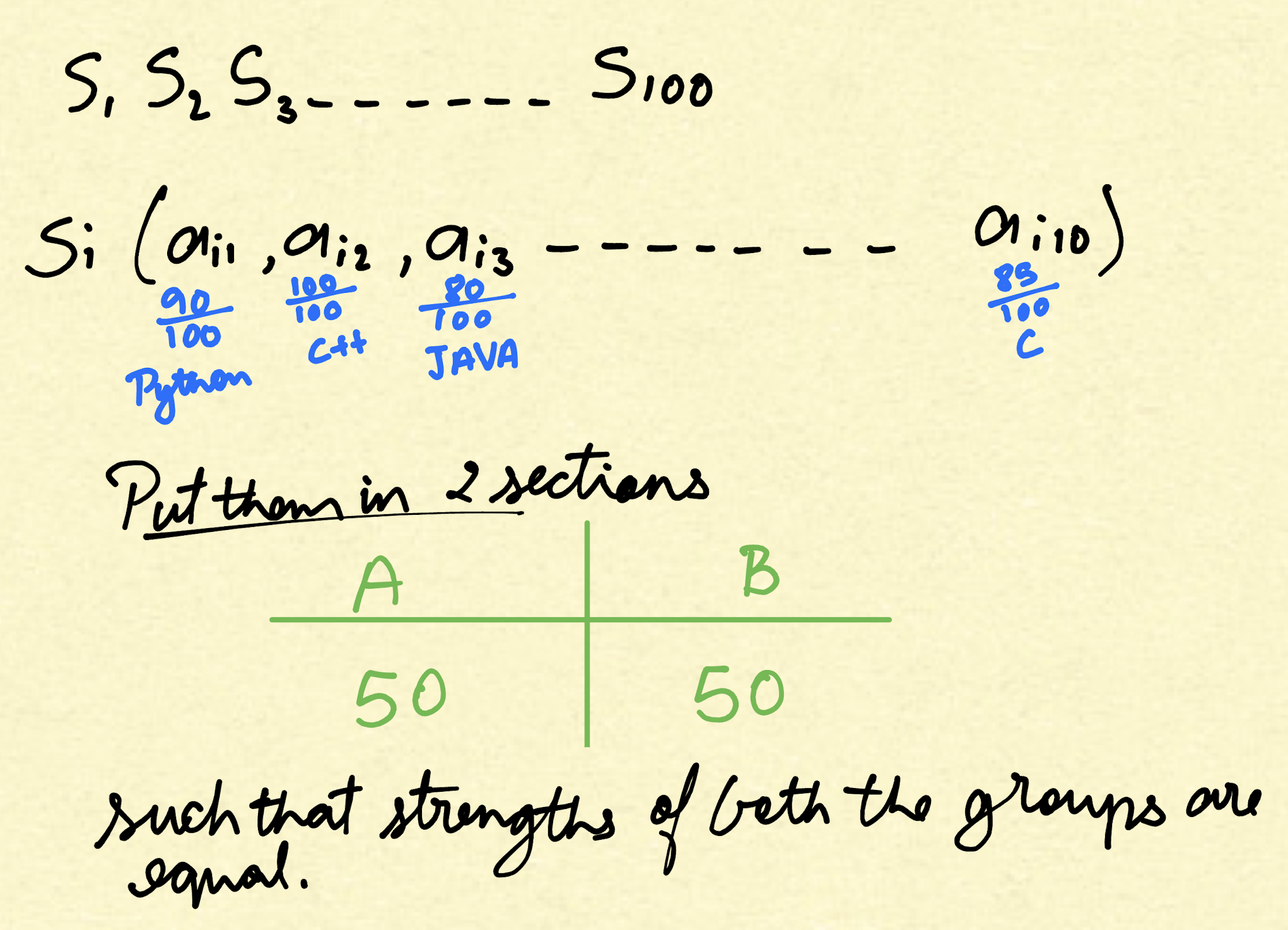
Project: A company has 100 employees, each rated in 10 distinct skills. Each employee’s rating in a skill reflects their experience, expertise, and comfort in that skill, with values ranging from 0 to 100. The company wants to divide its employees into two groups of 50 each, such that the total skill levels for each group are identical across all 10 skills.
Your task is to divide the employees into two equal-sized groups (50 each) such that for every skill, the sum of the skill ratings in Group 1 is equal to the sum of the skill ratings in Group 2.
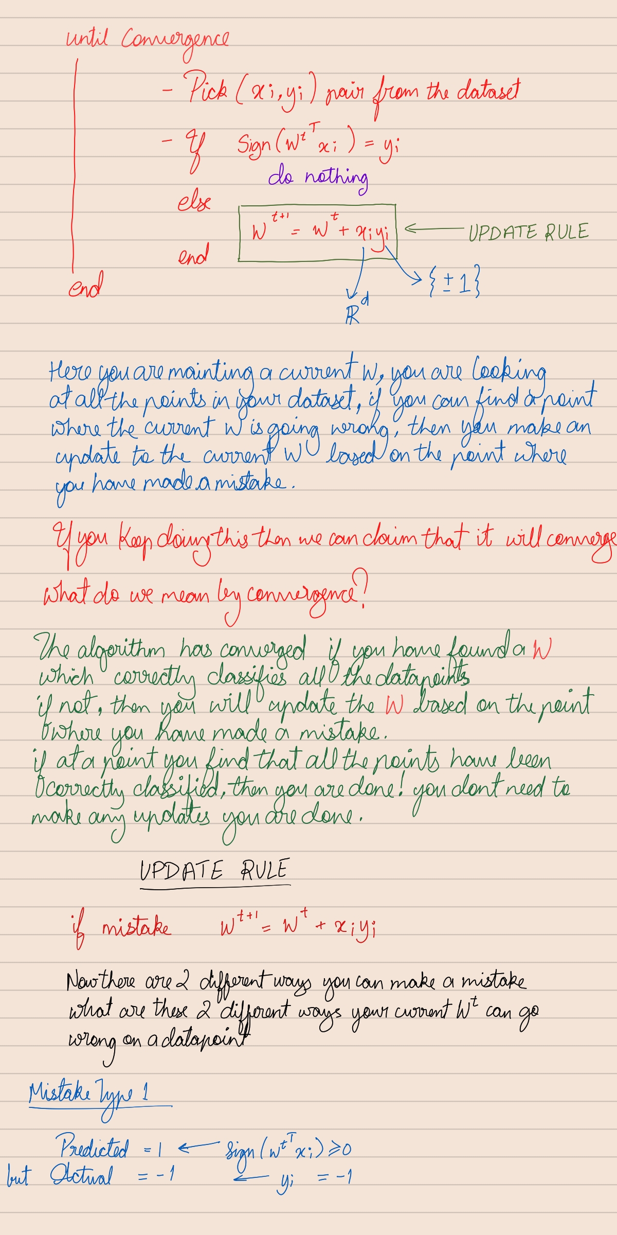
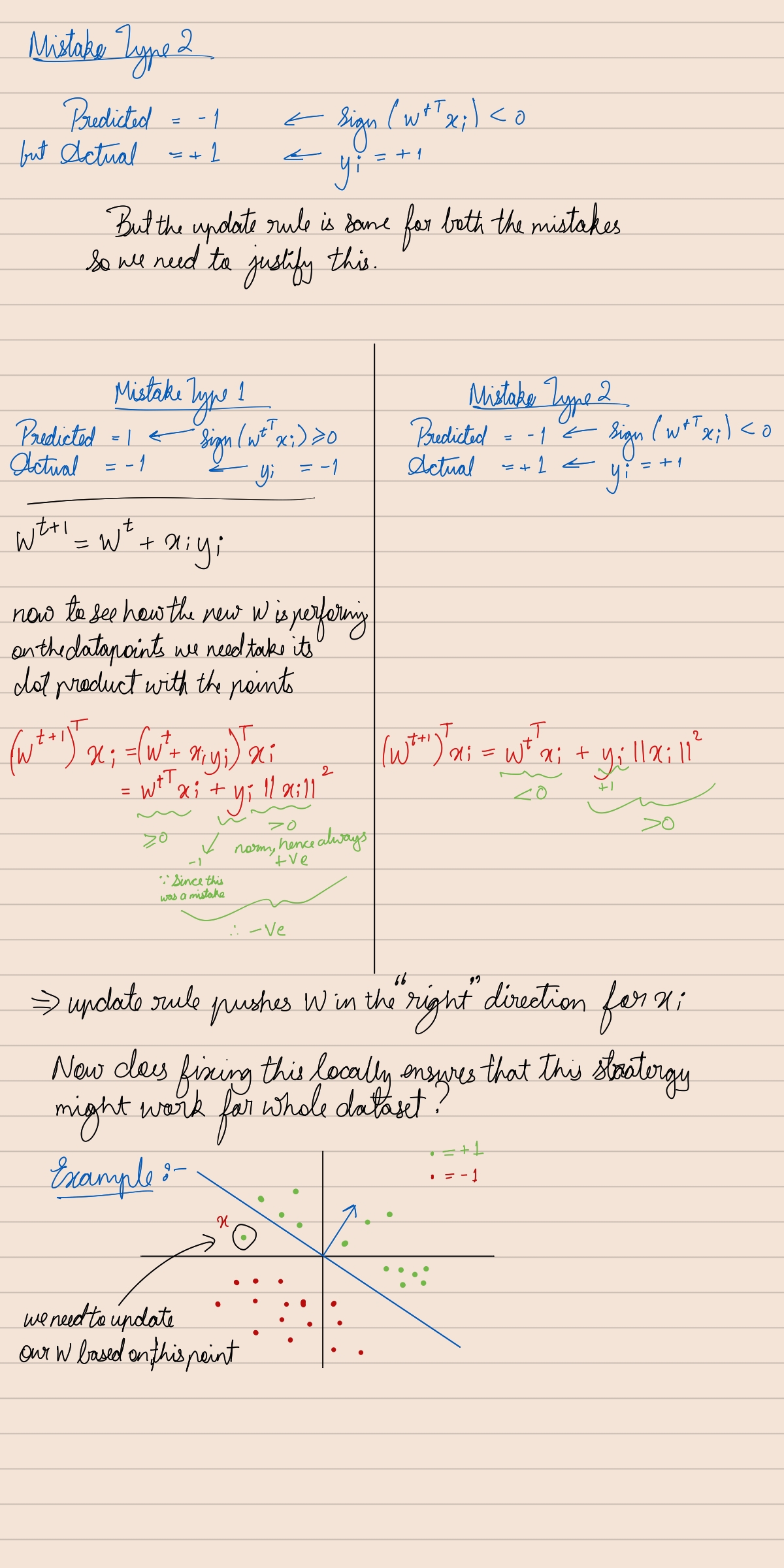
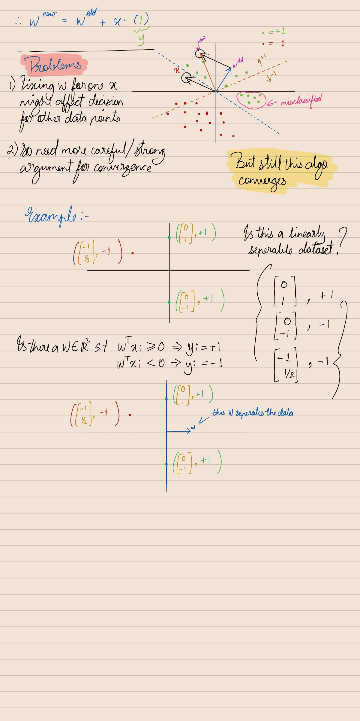
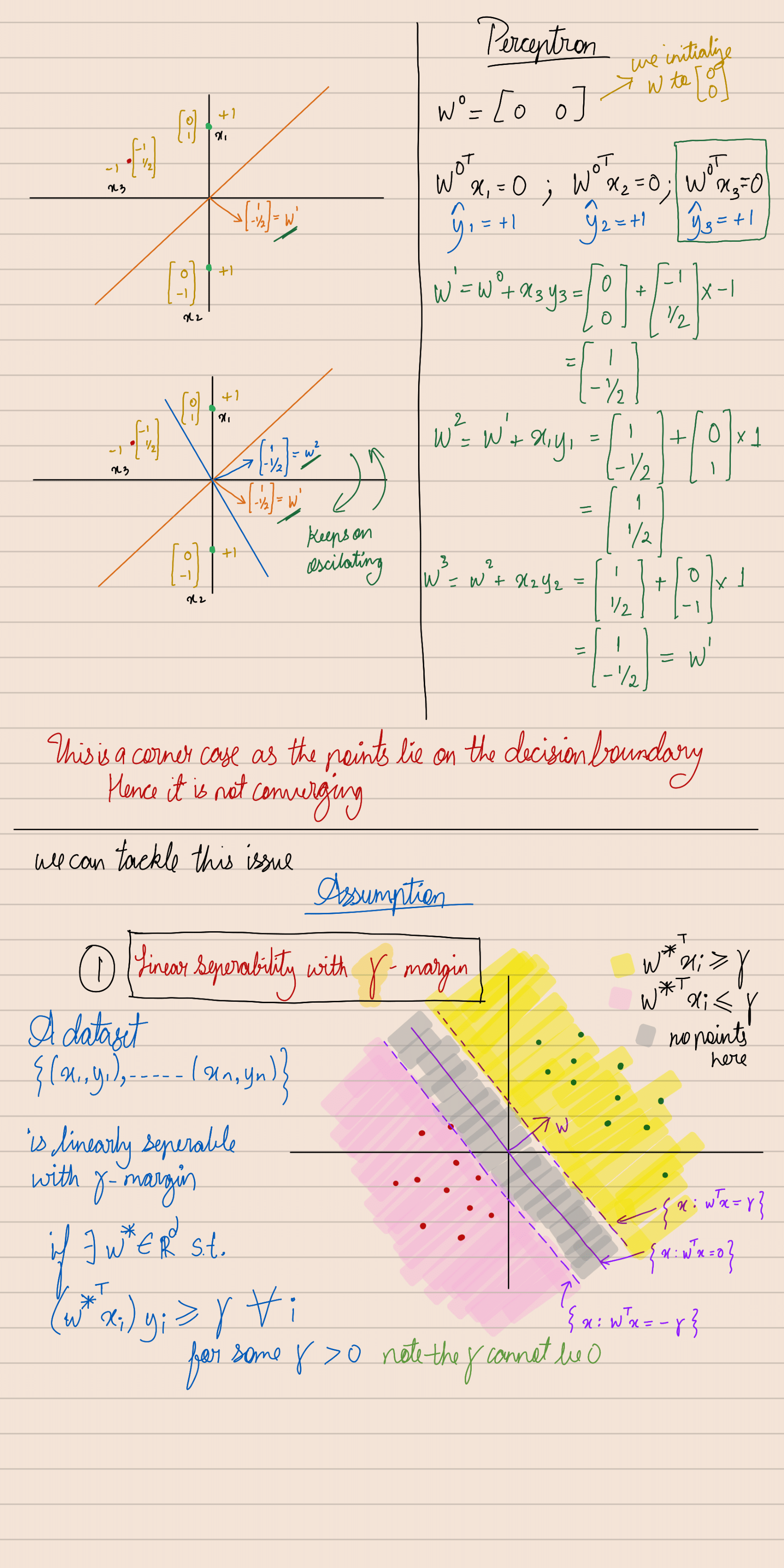
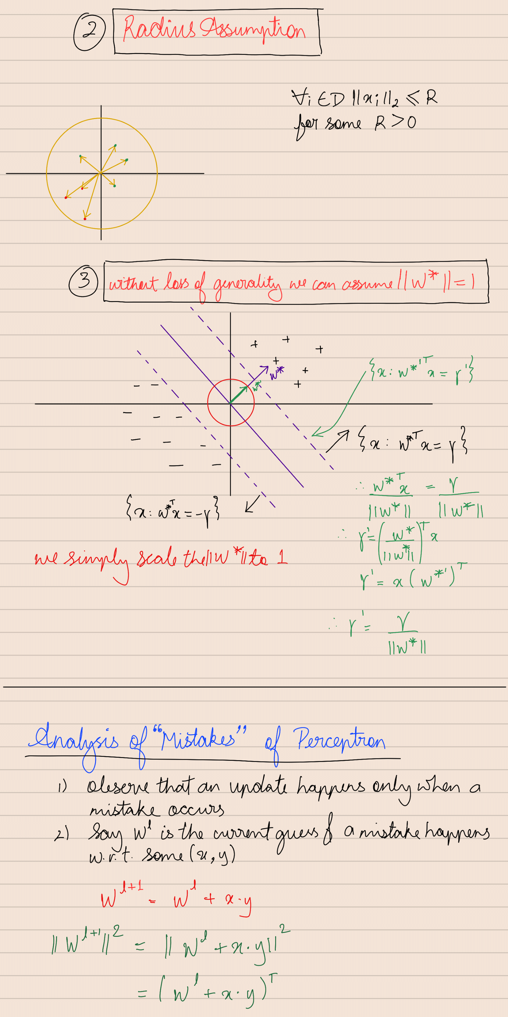
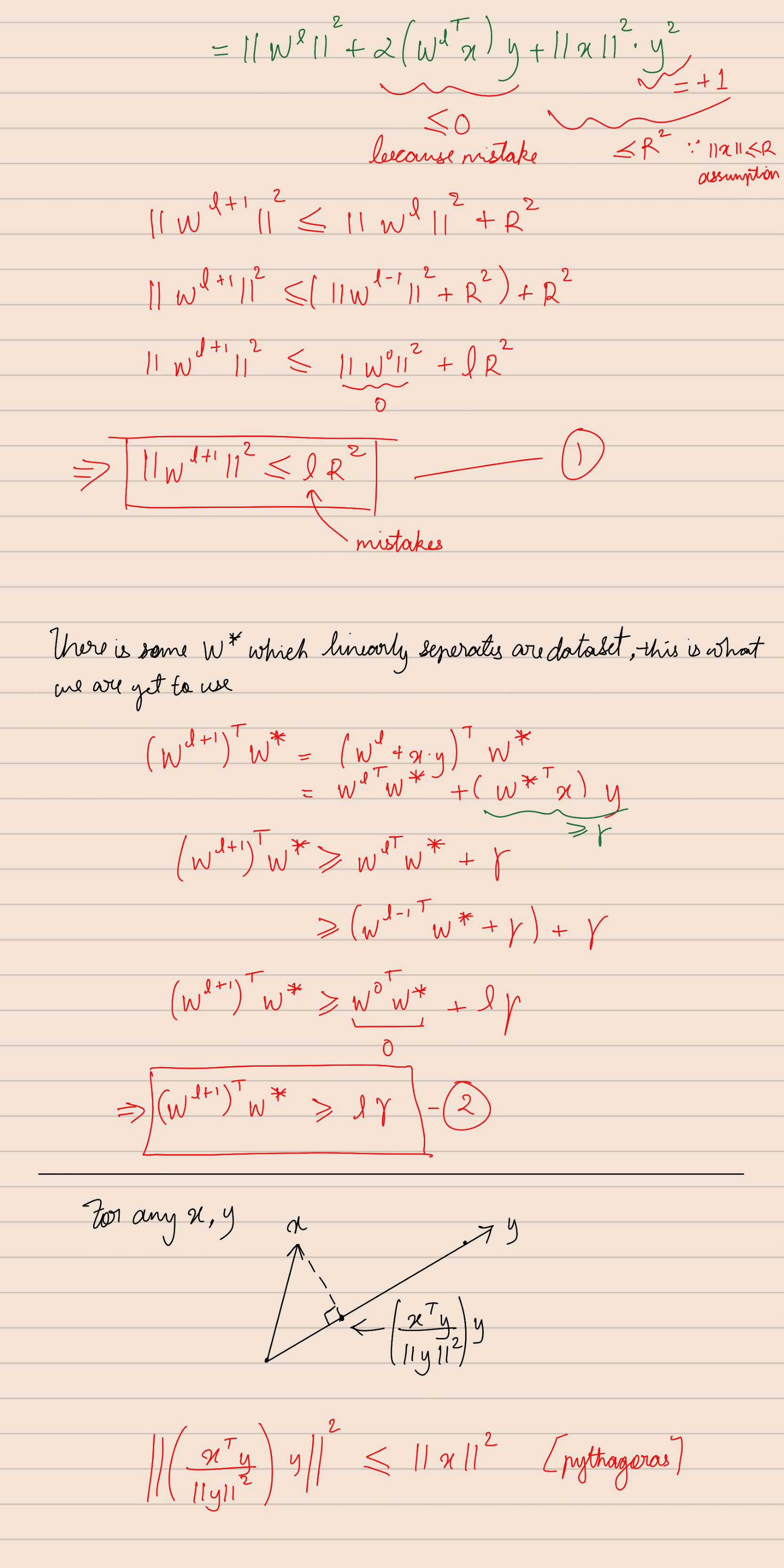
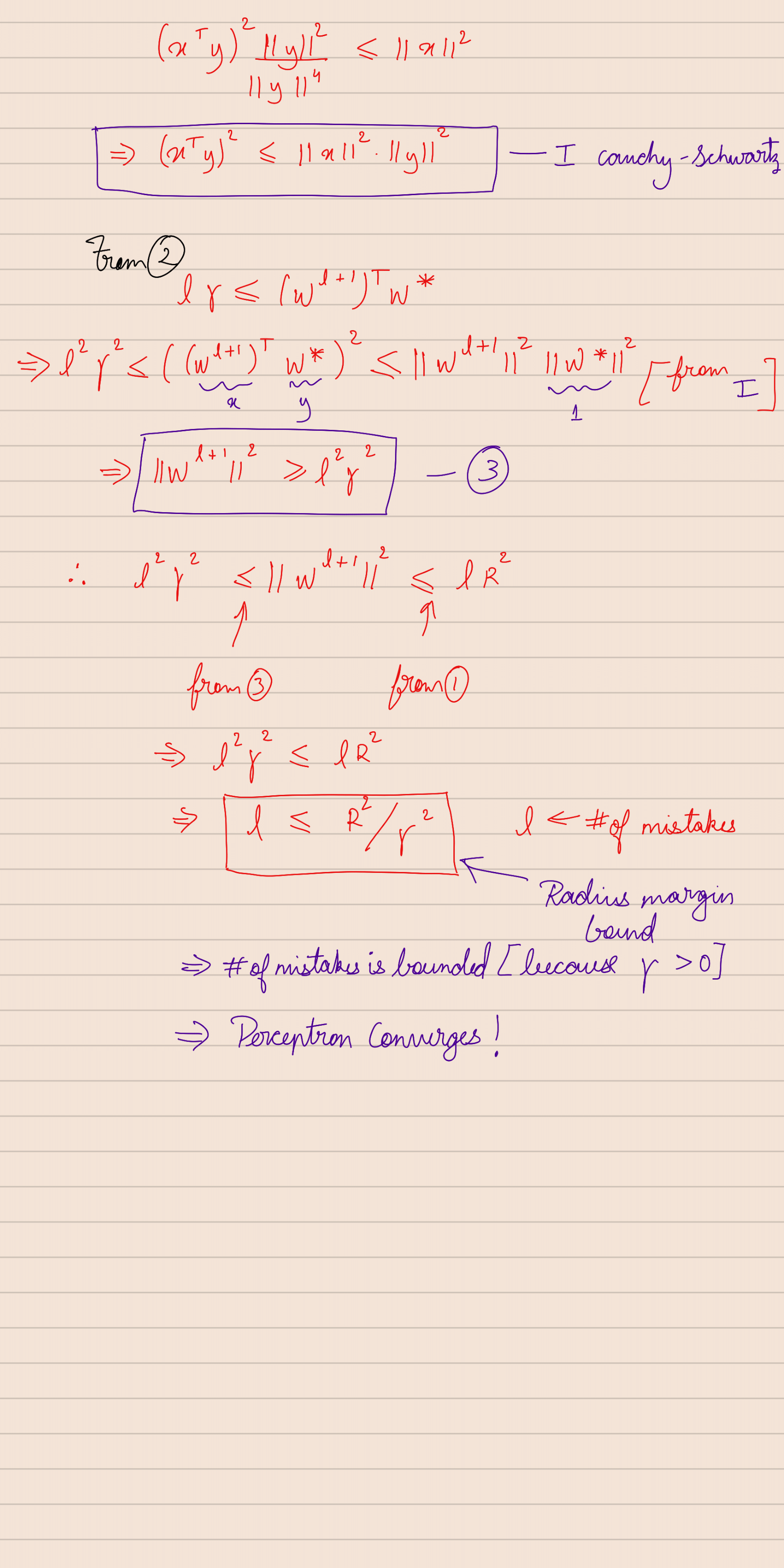
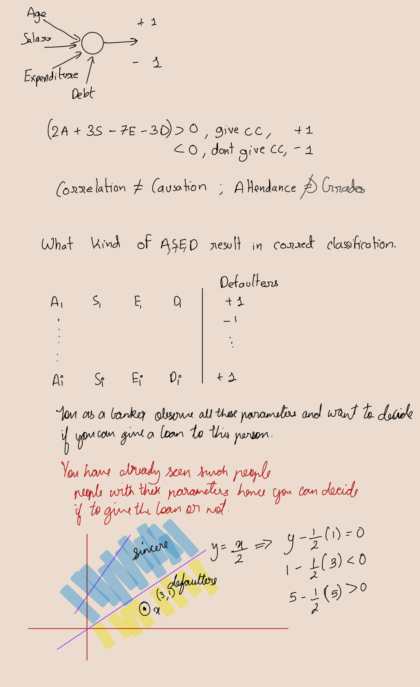
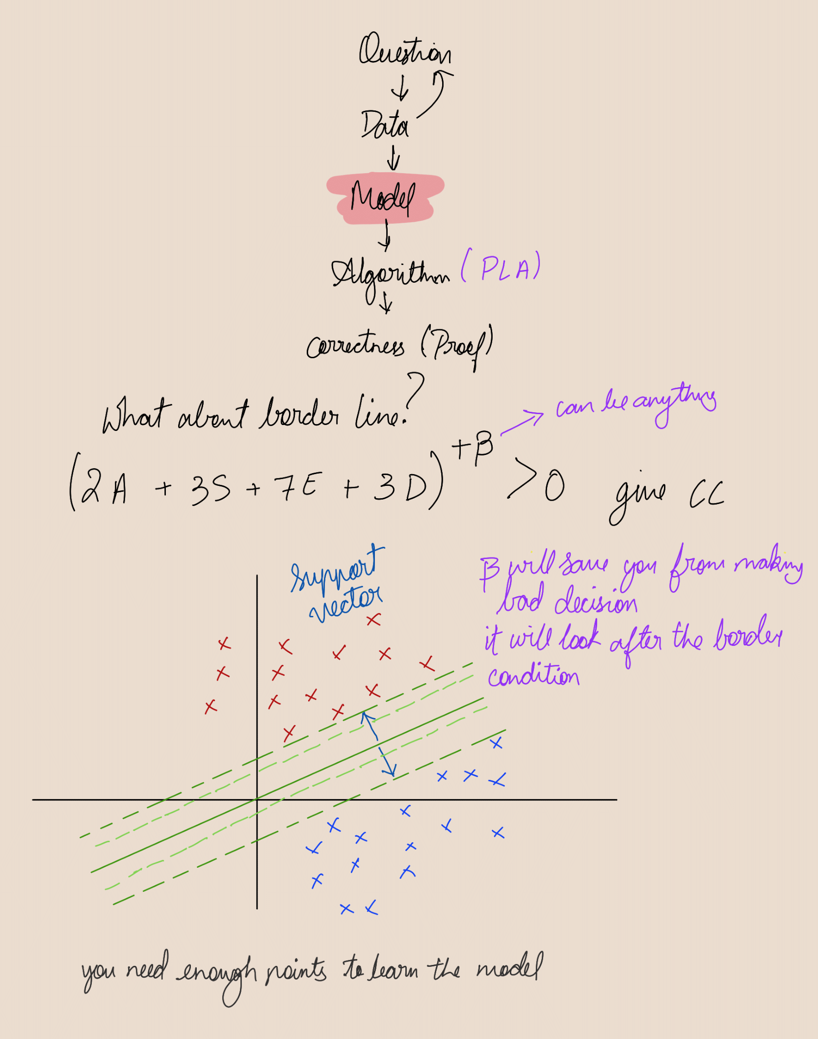
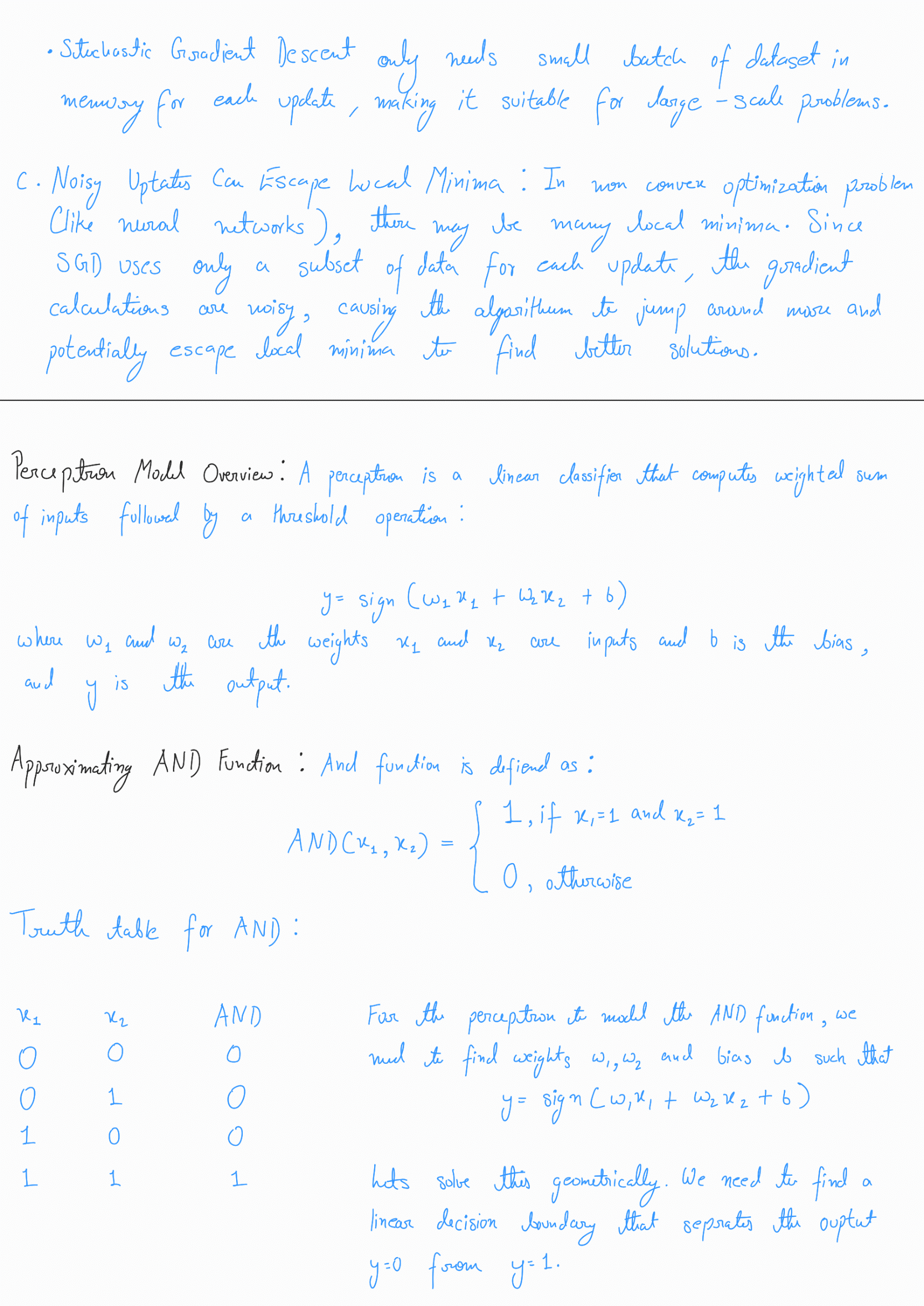
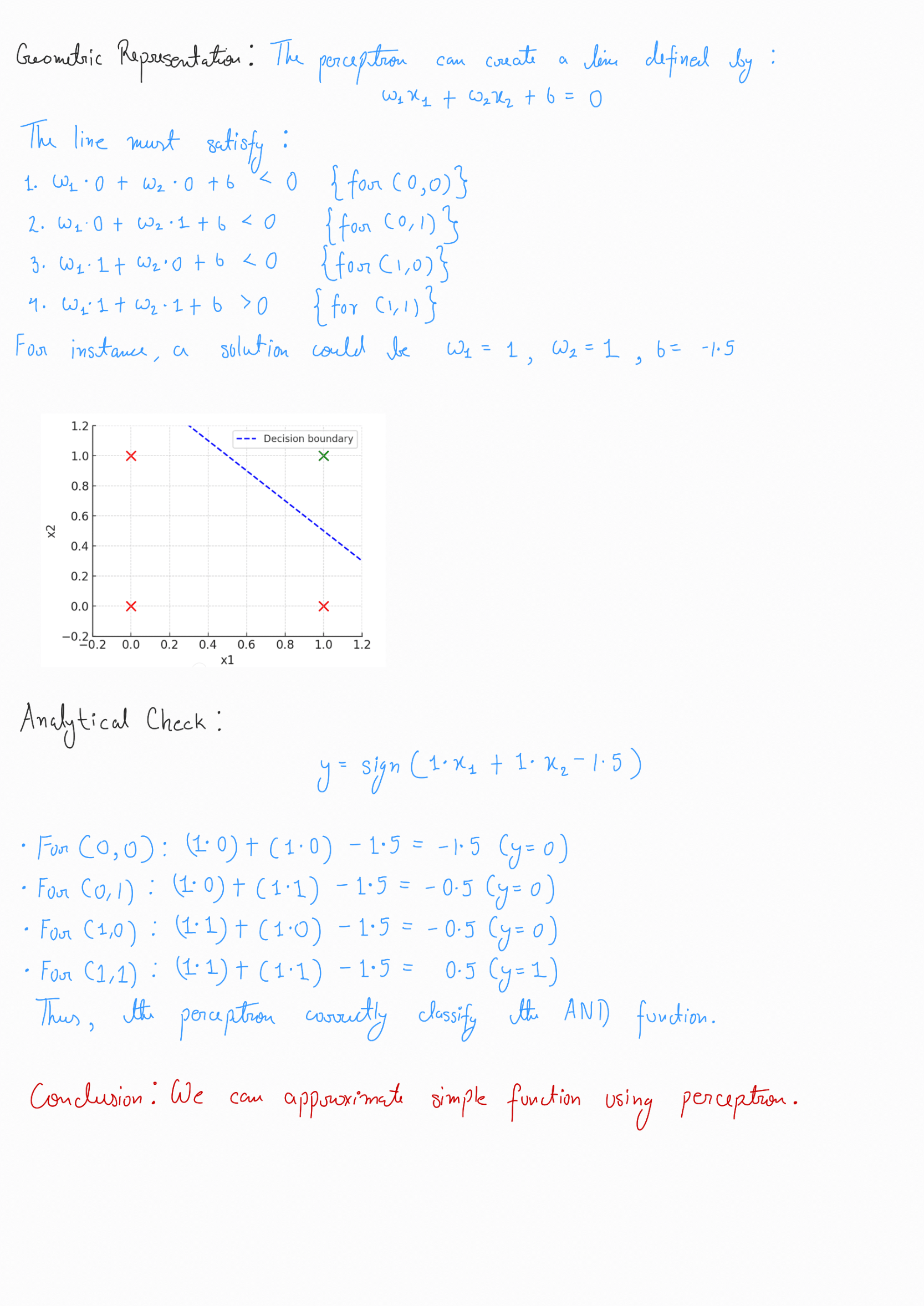
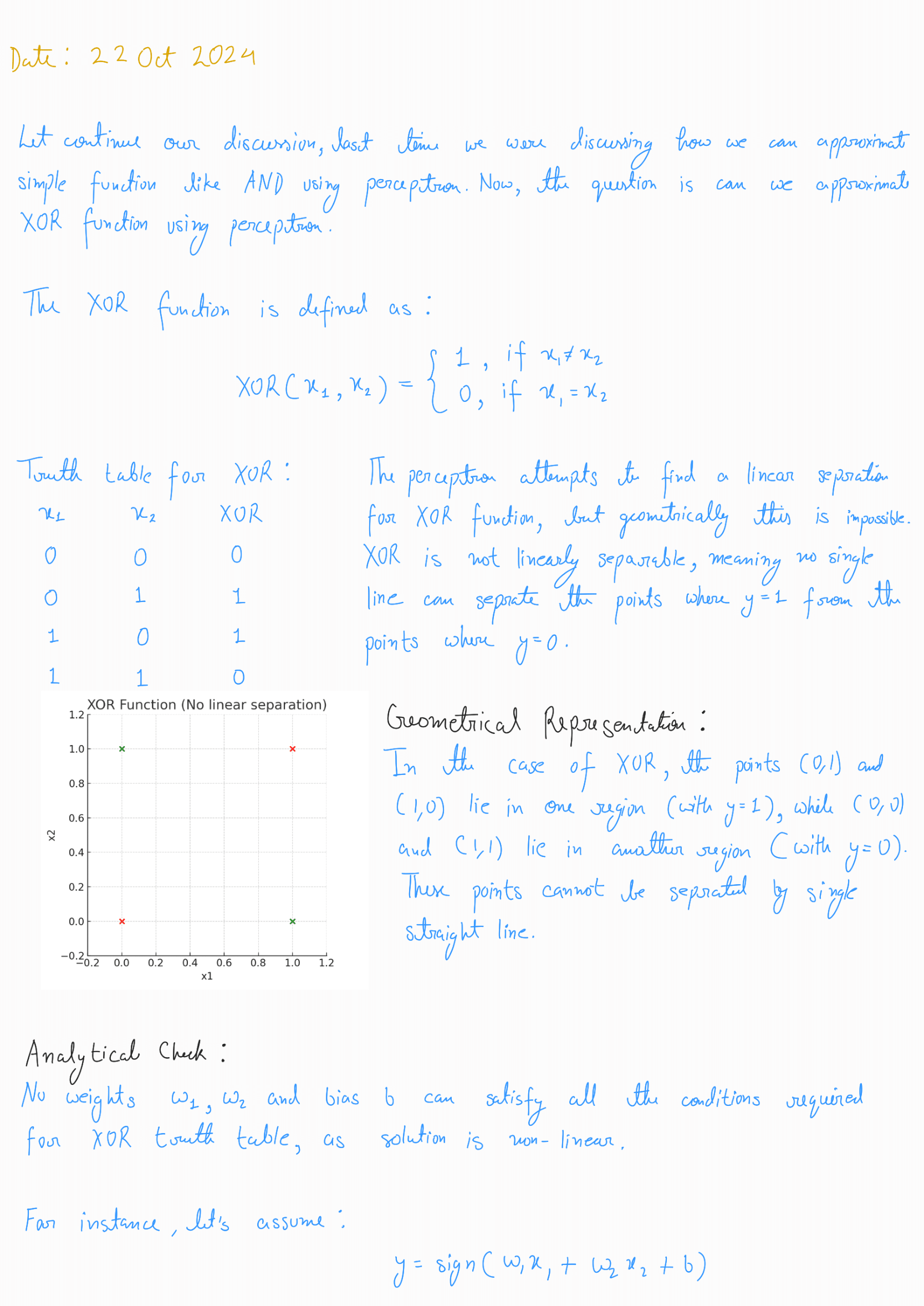
Perceptron Learning Algorithm
Update Rule
SVD

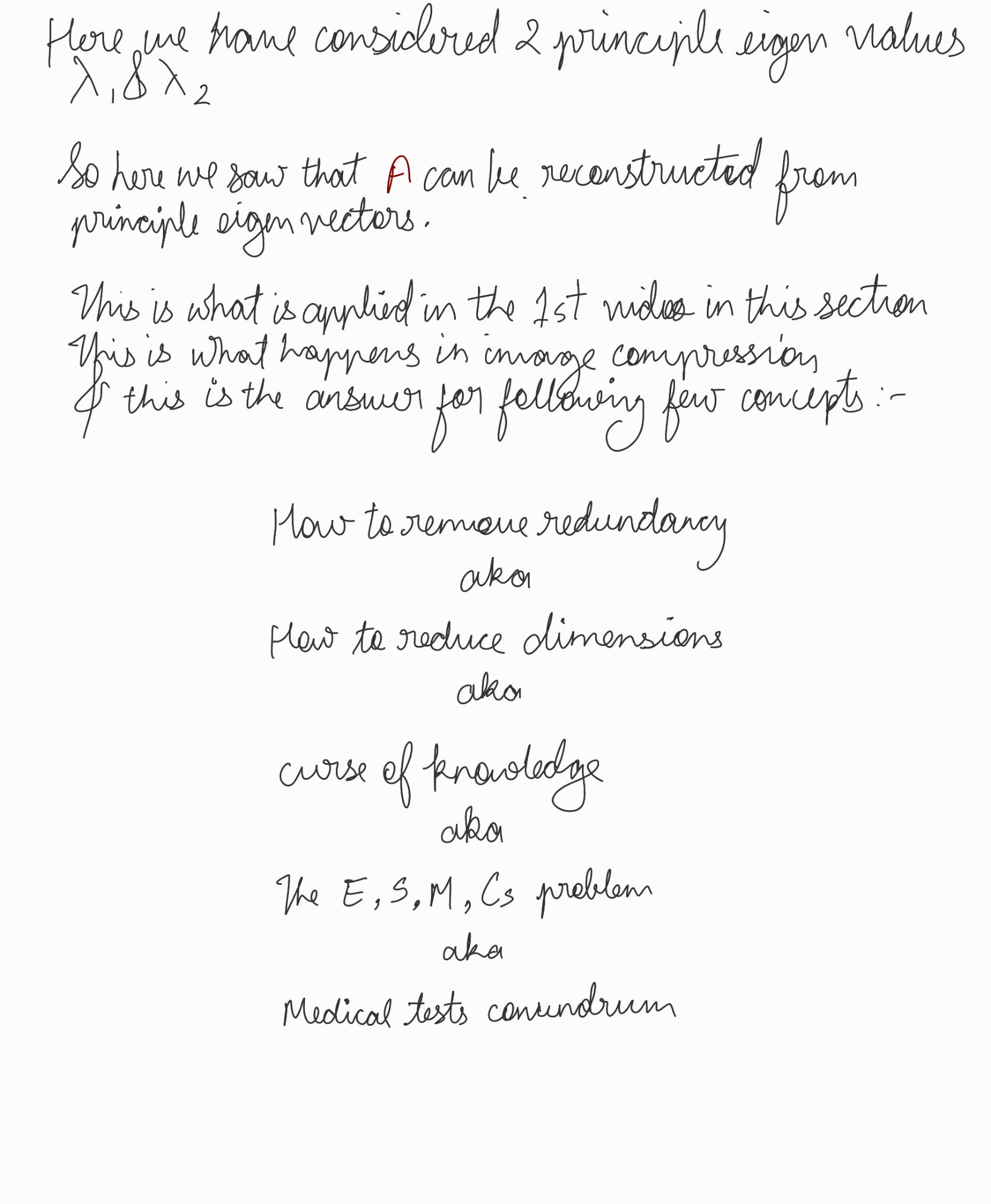
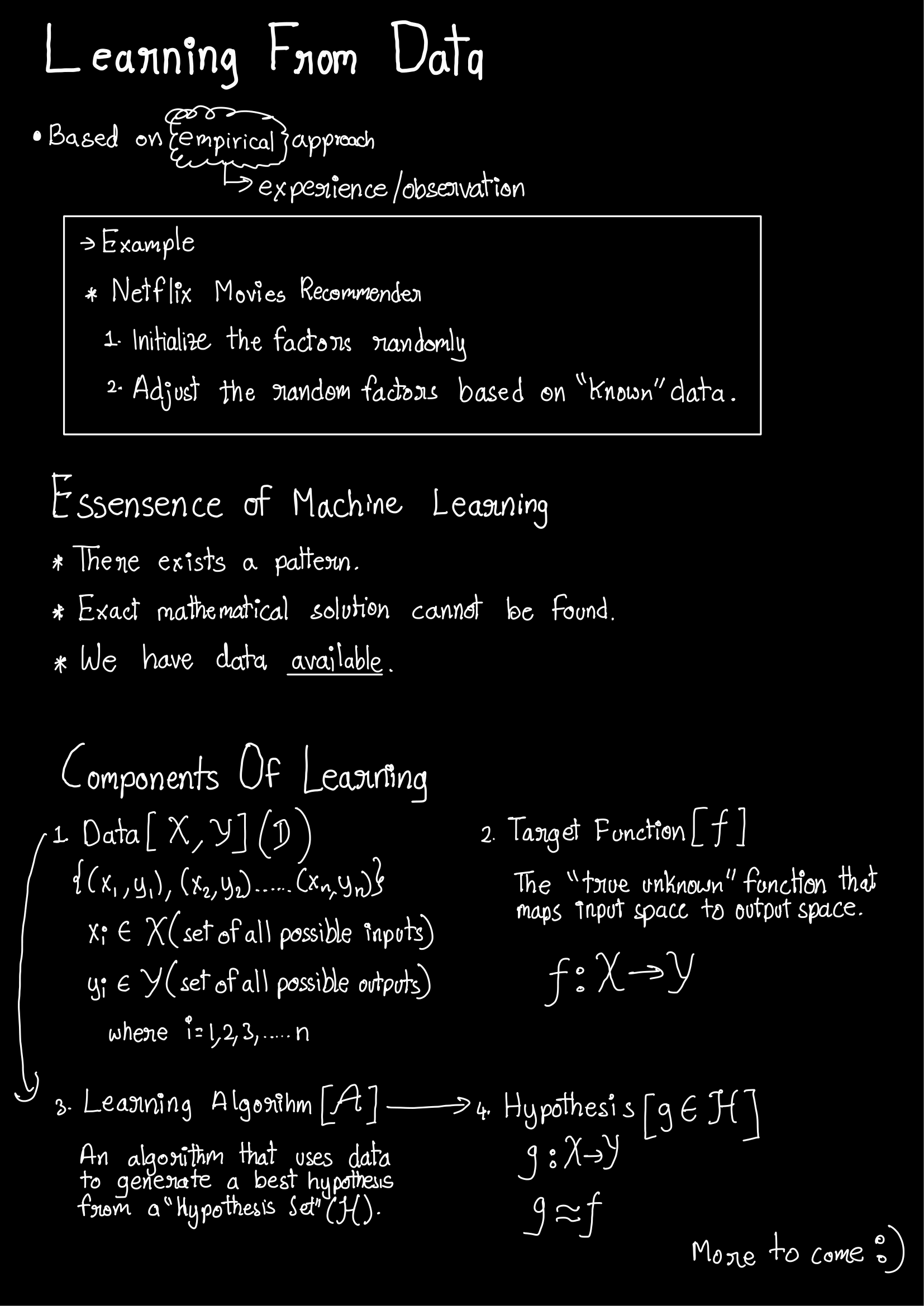
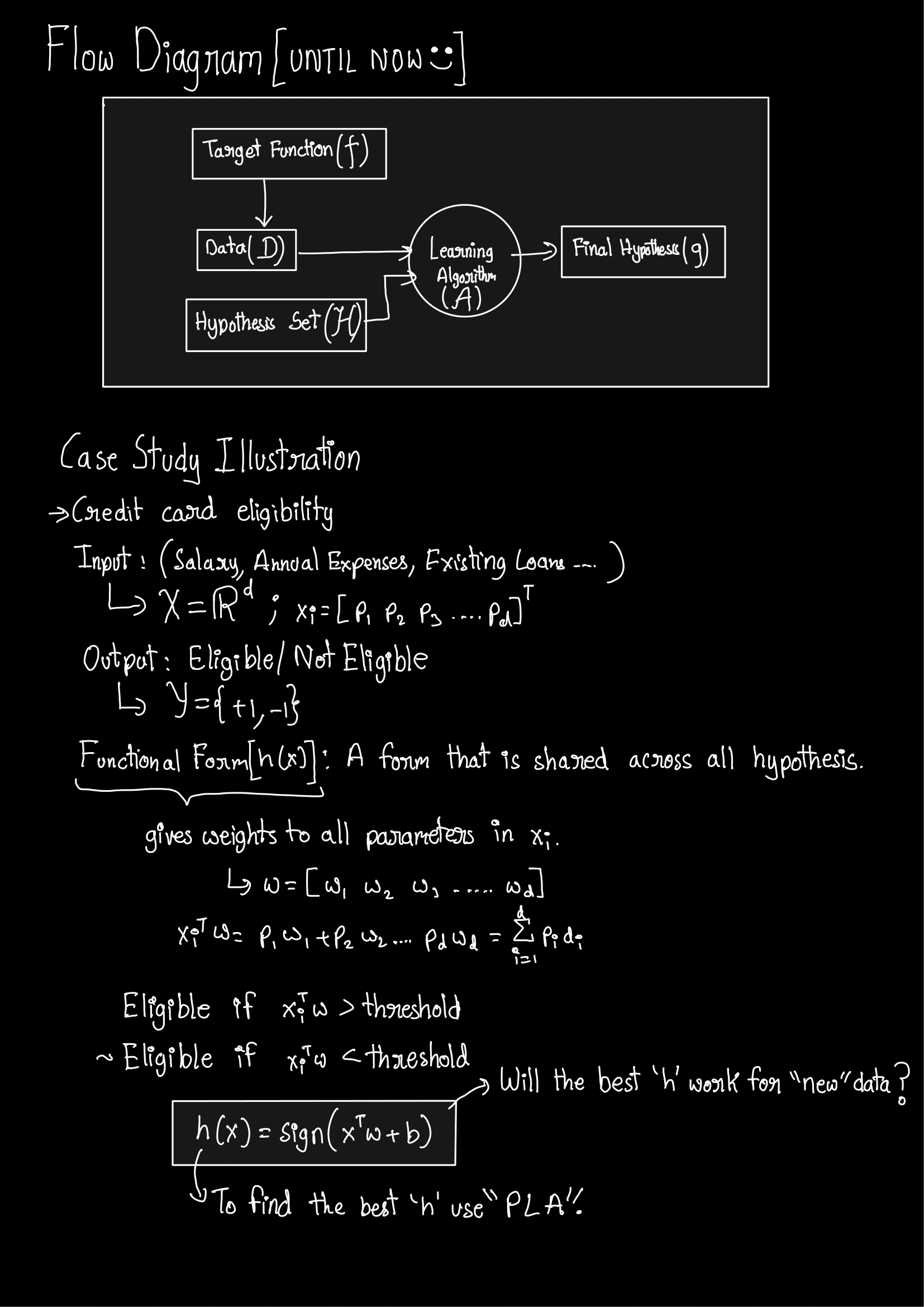
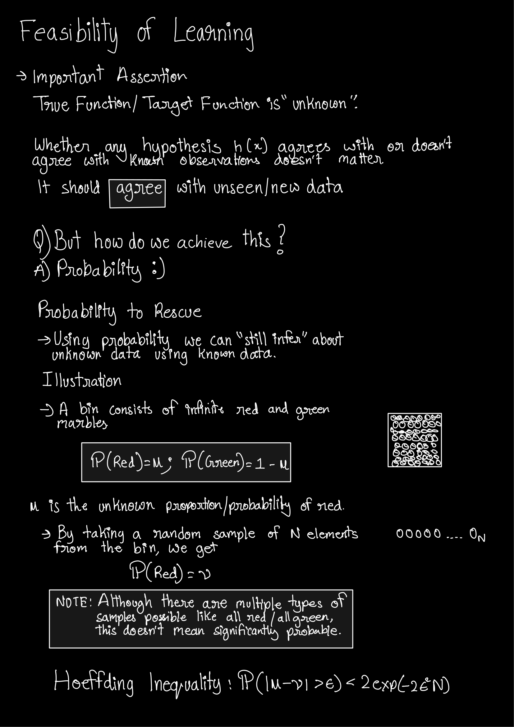
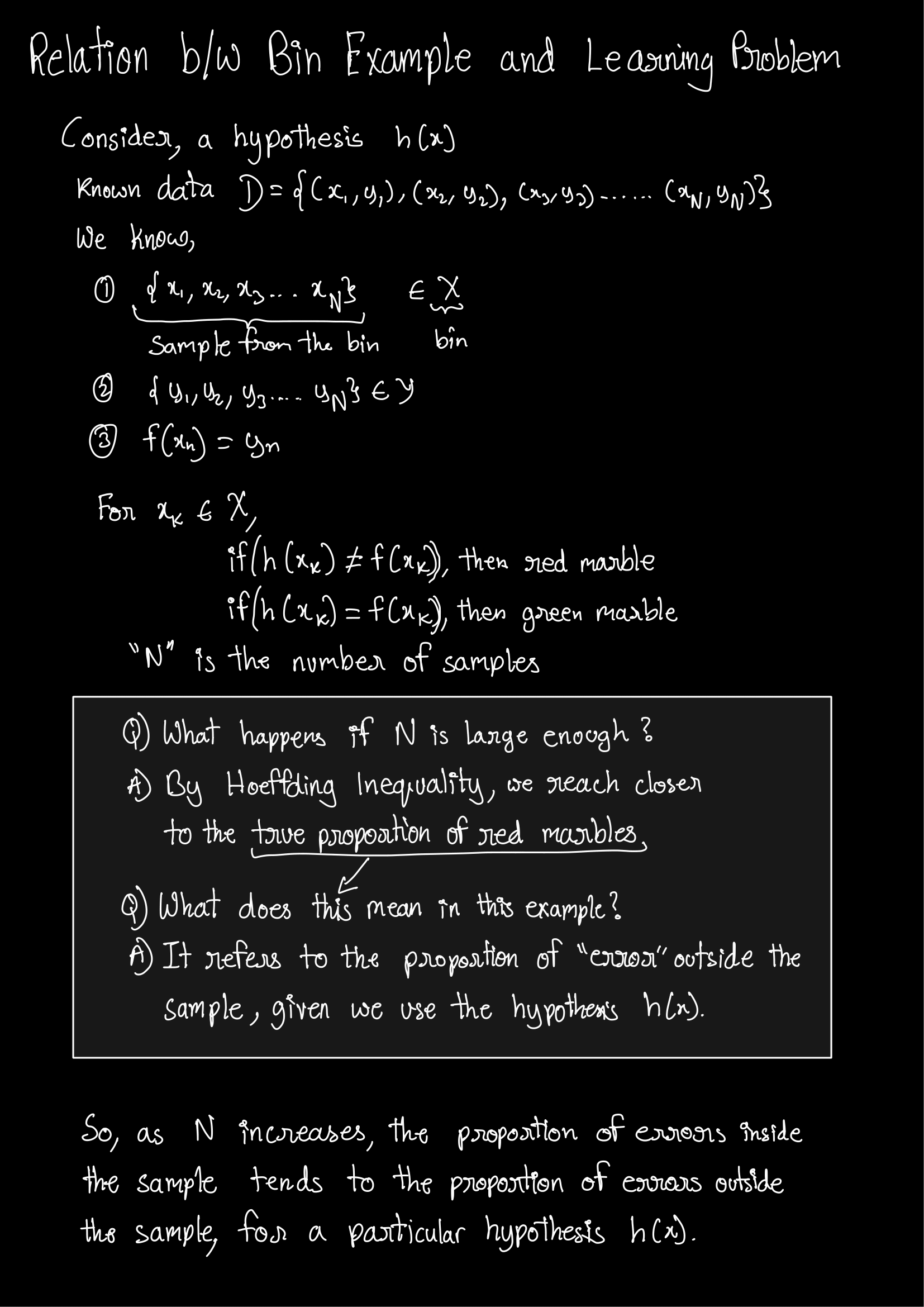
The Learning Problem
1. Recap of Previous Session
We began by recalling the major problem we were addressing:
- Goal: To understand how well a learned model (hypothesis) generalizes from the training data (in-sample) to new, unseen data (out-of-sample).
- Importance: It’s crucial to not only fit the training data but also to perform well on future data.
2. Sampling and Estimation
2.1. The Jar of Balls Analogy
- Scenario: A jar contains an unknown mix of black and white balls.
- Objective: Estimate the proportion of black and white balls.
- Method:
- Sampling: Draw balls randomly and note their colors.
- Sample Proportions: If you draw 9 balls and get 2 black and 7 white, the sample proportions are \(\frac{2}{9}\) black and \(\frac{7}{9}\) white.
- Inference:
- Use sample proportions to infer the true proportions in the jar.
- Law of Large Numbers: Increasing the number of samples improves the accuracy of the estimate.
2.2. Importance of Sample Size
- Reducing Variability: Larger samples reduce the probability that the sample estimate deviates significantly from the true proportion.
- Confidence in Estimates: More samples lead to tighter bounds on estimation errors.
3. Machine Learning Concepts
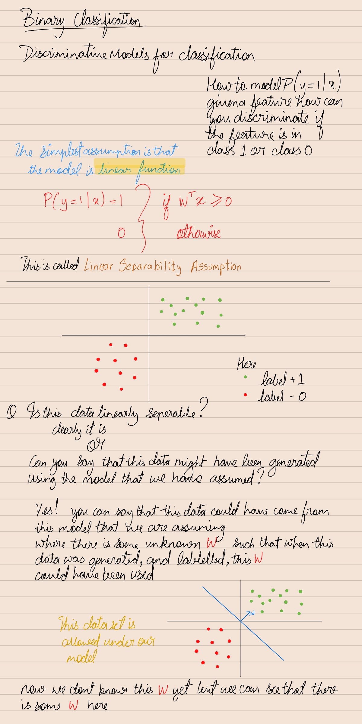
3.1. Hypothesis Functions and Classification
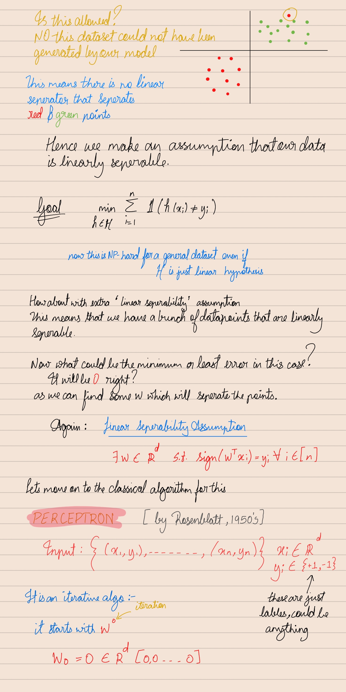
- Data Points: Consider a set of points to classify.
- Hypothesis Set (\(H\)):
- A collection of functions (classifiers) used to model the data.
- Examples: Linear classifiers, decision trees, neural networks.
- Redundancy in \(H\):
- Functions that classify data identically can be considered the same.
- Simplifying \(H\): Reduces complexity by eliminating redundant hypotheses.
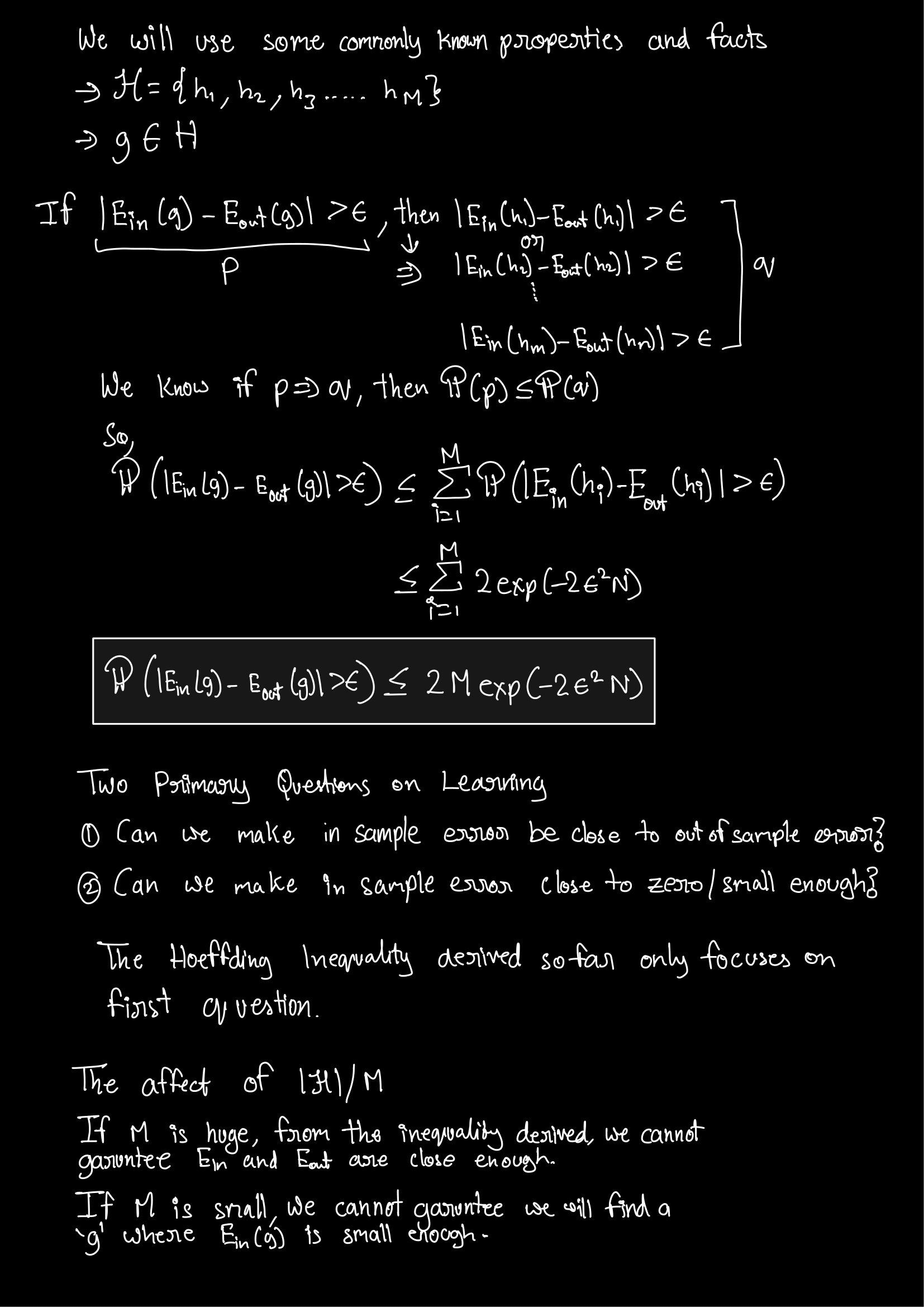
3.2. In-Sample and Out-of-Sample Error
- In-Sample Error (\(E_{\text{in}}\)):
- The proportion of misclassified points in the training data.
- Out-of-Sample Error (\(E_{\text{out}}\)):
- The expected error on new, unseen data.
- Goal: Minimize \(E_{\text{out}}\) to ensure good generalization.
4. Generalization and Error Bounds
4.1. The Need for Error Bounds
- Challenge: \(E_{\text{out}}\) cannot be directly computed.
- Solution: Use probabilistic bounds to relate \(E_{\text{in}}\) and \(E_{\text{out}}\).
- Key Question: How can we ensure that \(E_{\text{in}}\) is close to \(E_{\text{out}}\)?
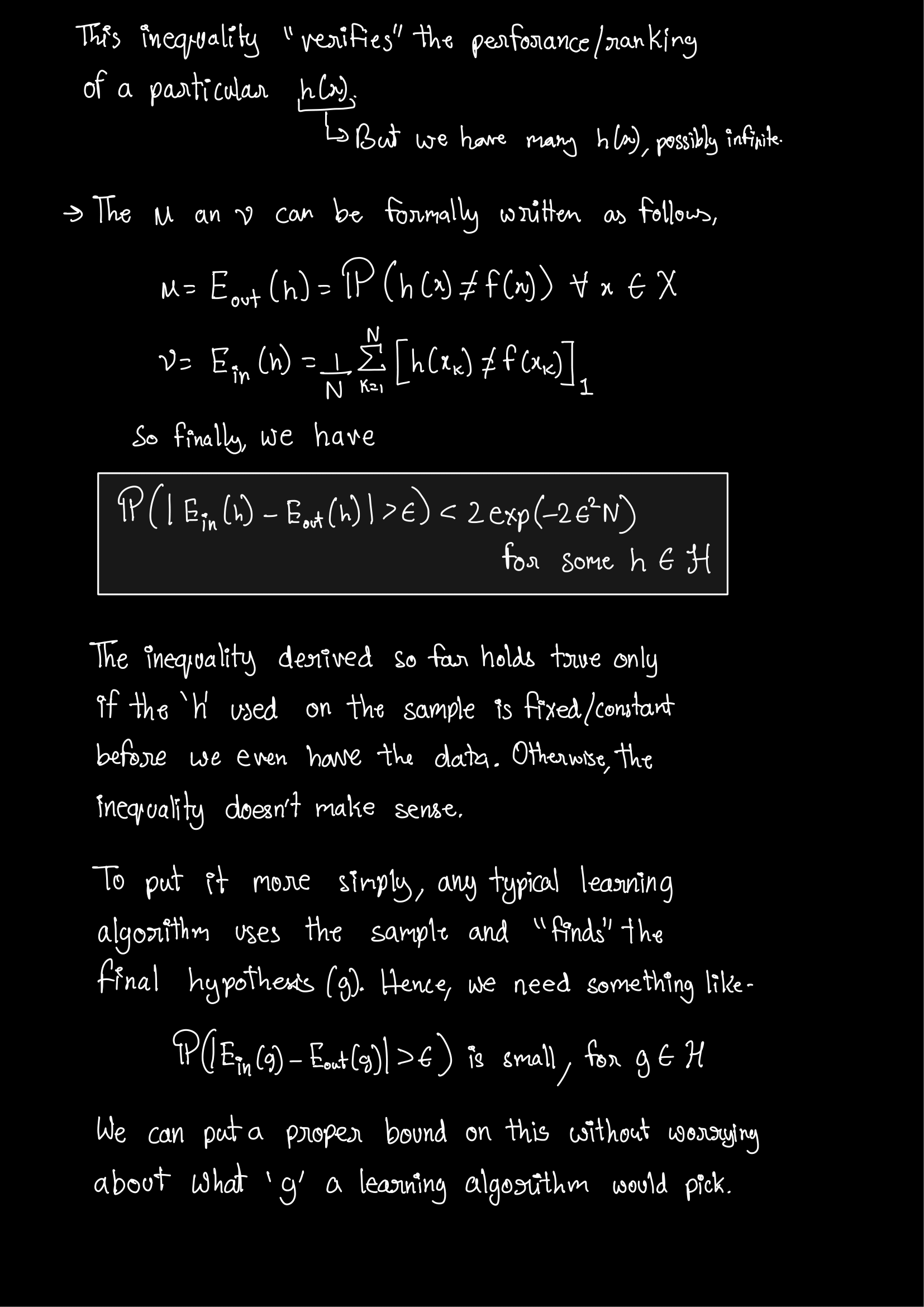
4.2. Hoeffding’s Inequality
- Statement:
- For independent random variables, the probability that the sample mean deviates from the true mean by more than \(\epsilon\) decreases exponentially with sample size (\(N\)).
- Formula: \(P\left(|E_{\text{in}} - E_{\text{out}}| > \epsilon\right) \leq 2e^{-2\epsilon^2 N}\)
- Interpretation:
- Provides a bound on the probability that the in-sample error deviates from the out-of-sample error.
4.3. Union Bound
- Concept:
- When considering multiple hypotheses, the probability that any one of them fails to generalize well is bounded by the sum of their individual probabilities.
- Application:
- For \(M\) hypotheses: \(P\left(\exists h \in H: |E_{\text{in}}(h) - E_{\text{out}}(h)| > \epsilon\right) \leq 2M e^{-2\epsilon^2 N}\)
- Implication:
- The more hypotheses we have, the looser the bound becomes unless \(N\) increases.
5. The Role of Hypothesis Complexity
5.1. Number of Hypotheses (\(M\))
- Effect on Error Bounds:
- Larger \(M\) increases the bound, making it harder to guarantee small \(E_{\text{out}}\).
- Managing Complexity:
- Limiting \(M\) (e.g., through regularization) helps improve generalization.
5.2. VC Dimension
- Definition:
- A measure of the capacity of a hypothesis set to shatter datasets.
- Significance:
- Higher VC dimension implies the ability to fit more complex patterns but risks overfitting.
- Balancing Act:
- Choose models with appropriate VC dimensions relative to the sample size.
6. Practical Examples
6.1. Coin Toss Experiment
- Setup:
- Six people each toss a coin 1,000 times.
- Record the number of heads for each person.
- Analysis:
- Expected Heads: Approximately 500 heads per person.
- Minimum Number of Heads:
- The probability of any one person getting significantly fewer heads is low.
- Calculating the minimum across multiple trials illustrates tail probabilities.
- Connection to Learning:
- Analogous to considering the worst-case hypothesis in a hypothesis set.
6.2. Height Distribution Analogy
- Observation:
- In a group of 100 students, finding a six-footer is probable.
- In larger groups, more extreme heights become observable.
- Relevance:
- Outliers can significantly impact statistical estimates.
- Highlights the importance of considering sample size in probability estimates.
7. Mathematical Derivations
7.1. Bounding the Error
- Objective:
- Find \(\epsilon\) such that \(P(\|E_{\text{in}} - E_{\text{out}}\| > \epsilon)\) is acceptably low.
- Derivation:
- Rearranging Hoeffding’s inequality to solve for \(\epsilon\): \(\epsilon = \sqrt{\frac{\ln(2M/\delta)}{2N}}\) where \(\delta\) is the desired probability bound.
7.2. Understanding \(M\)
- Combinatorial Considerations:
- \(M\) can be large (even exponential) depending on the hypothesis set.
- Example:
- For binary classification with \(N\) points, \(M\) can be up to \(2^{N}\).
- Practical Approach:
- Use simpler models or regularization to keep \(M\) manageable.
- Ensures that the bound remains meaningful.
8. Key Insights and Takeaways
8.1. Balancing Sample Size and Model Complexity
- Sample Size (\(N\)):
- Increasing \(N\) tightens the error bound.
- Model Complexity (\(M\)):
- Reducing \(M\) (simpler models) also tightens the bound.
- Trade-Off:
- Need to balance complexity and available data to achieve good generalization.
8.2. Importance of Theoretical Understanding
- Mathematical Foundations:
- Provides confidence in the learning algorithms.
- Helps in designing models that generalize well.
- Practical Application:
- Use bounds and complexity measures to guide model selection and training.
9. Assignments and Further Reading
9.1. Upcoming Test
- Content:
- Based on the first five lectures from “Learning from Data” by Yaser S. Abu-Mostafa.
- Preparation:
- Watch the lectures available on YouTube.
- Review the corresponding chapters in the book.
9.2. Suggested Exercises
- Probability Calculations:
- Practice calculating bounds using Hoeffding’s inequality.
- Union Bound Applications:
- Solve problems involving multiple hypotheses and error probabilities.
- Understanding VC Dimension:
- Explore examples to compute the VC dimension of different hypothesis sets.
Summary
Understanding the theoretical aspects of machine learning is crucial for:
- Building Robust Models: Ensuring they perform well on unseen data.
- Avoiding Overfitting: Balancing complexity and generalization.
- Making Informed Decisions: Using mathematical bounds to guide the learning process.
As we continue, focus on internalizing these concepts and applying them to practical scenarios.
SVM
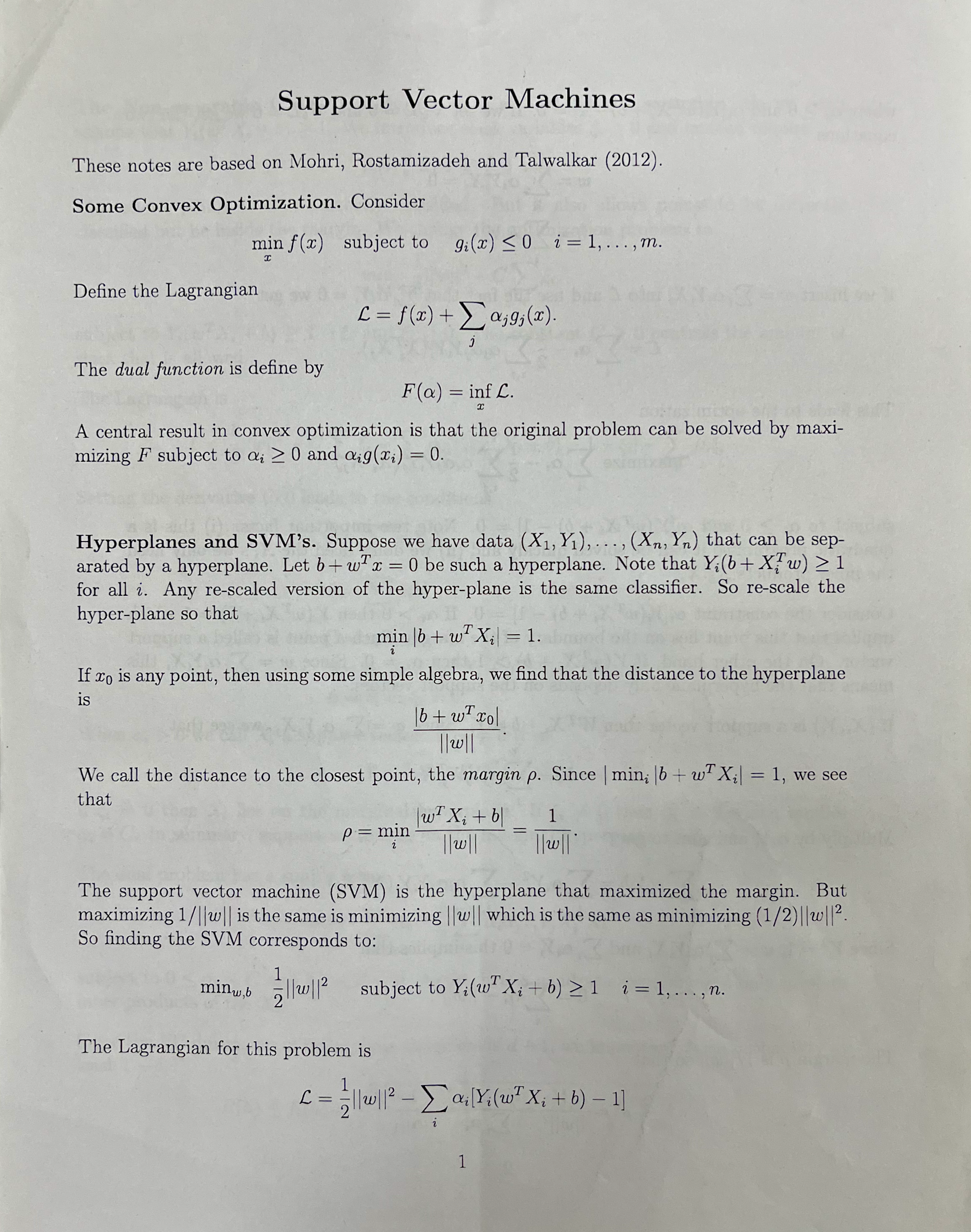
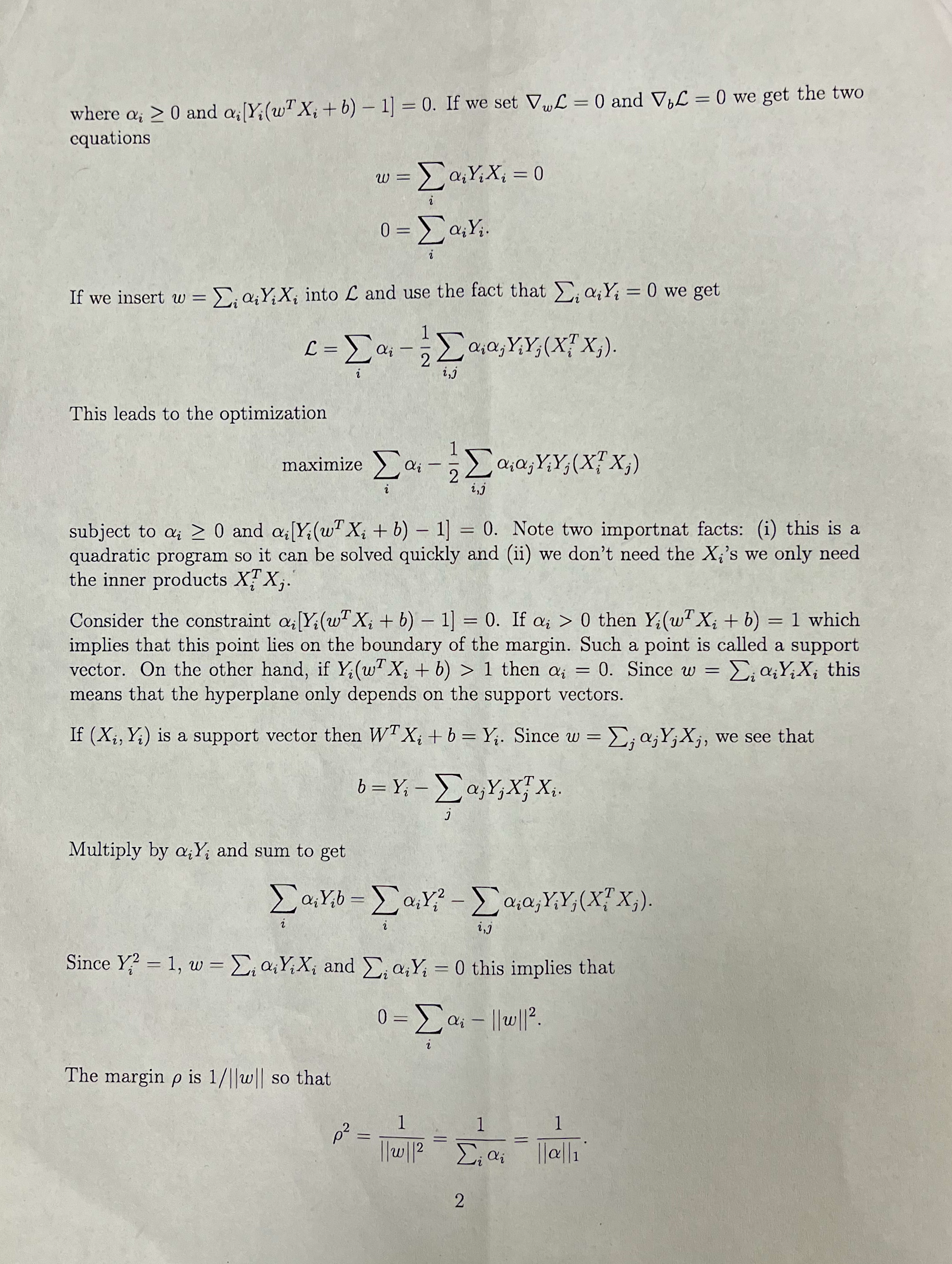
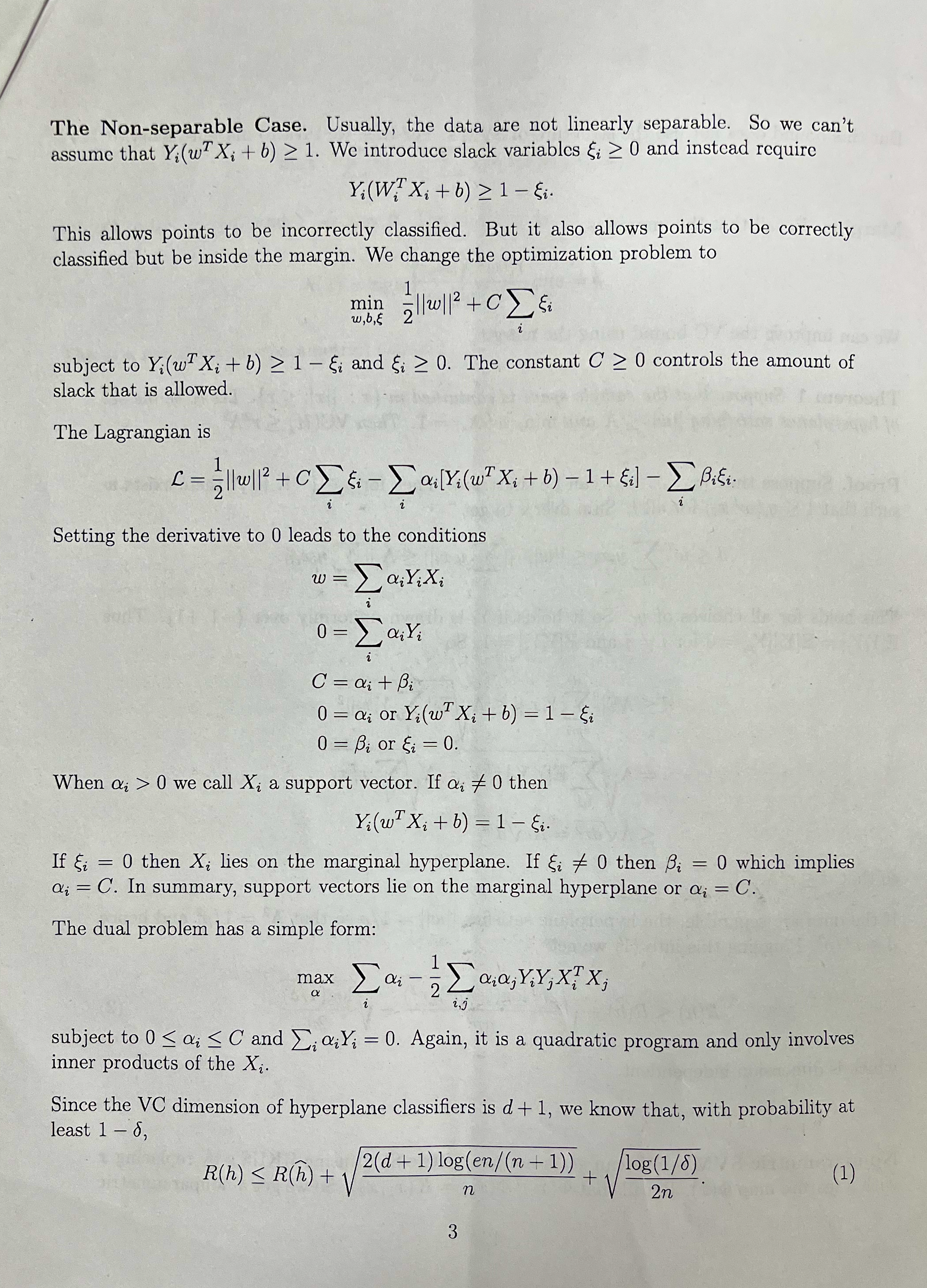
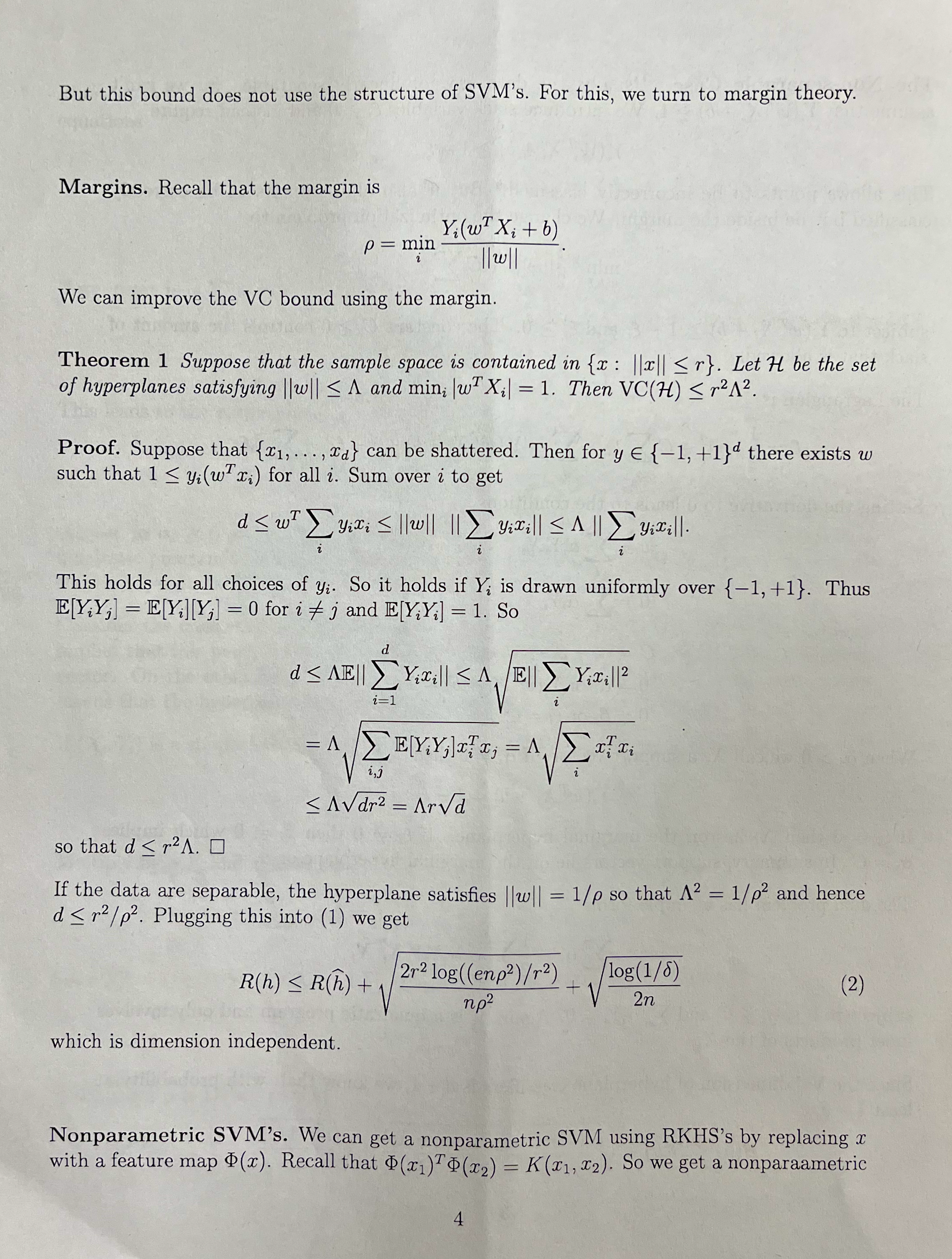
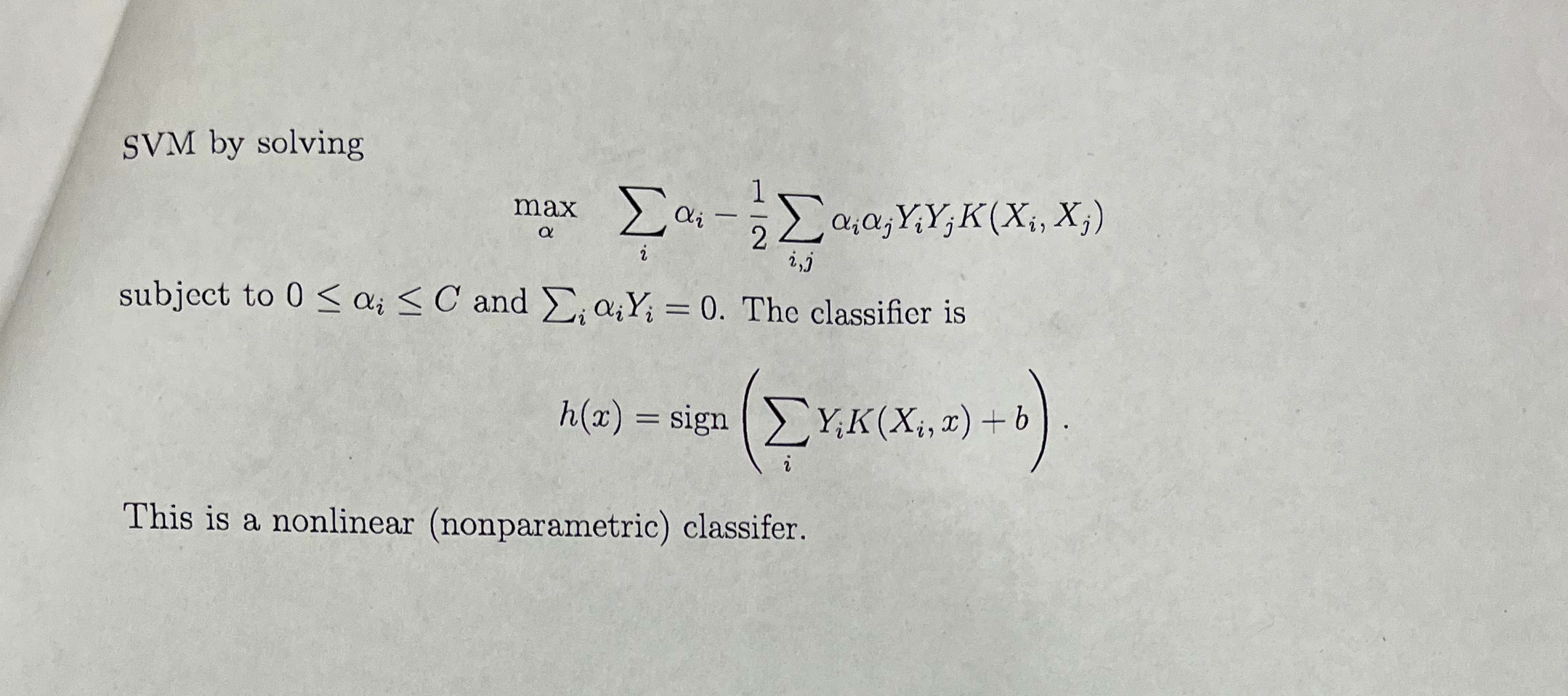
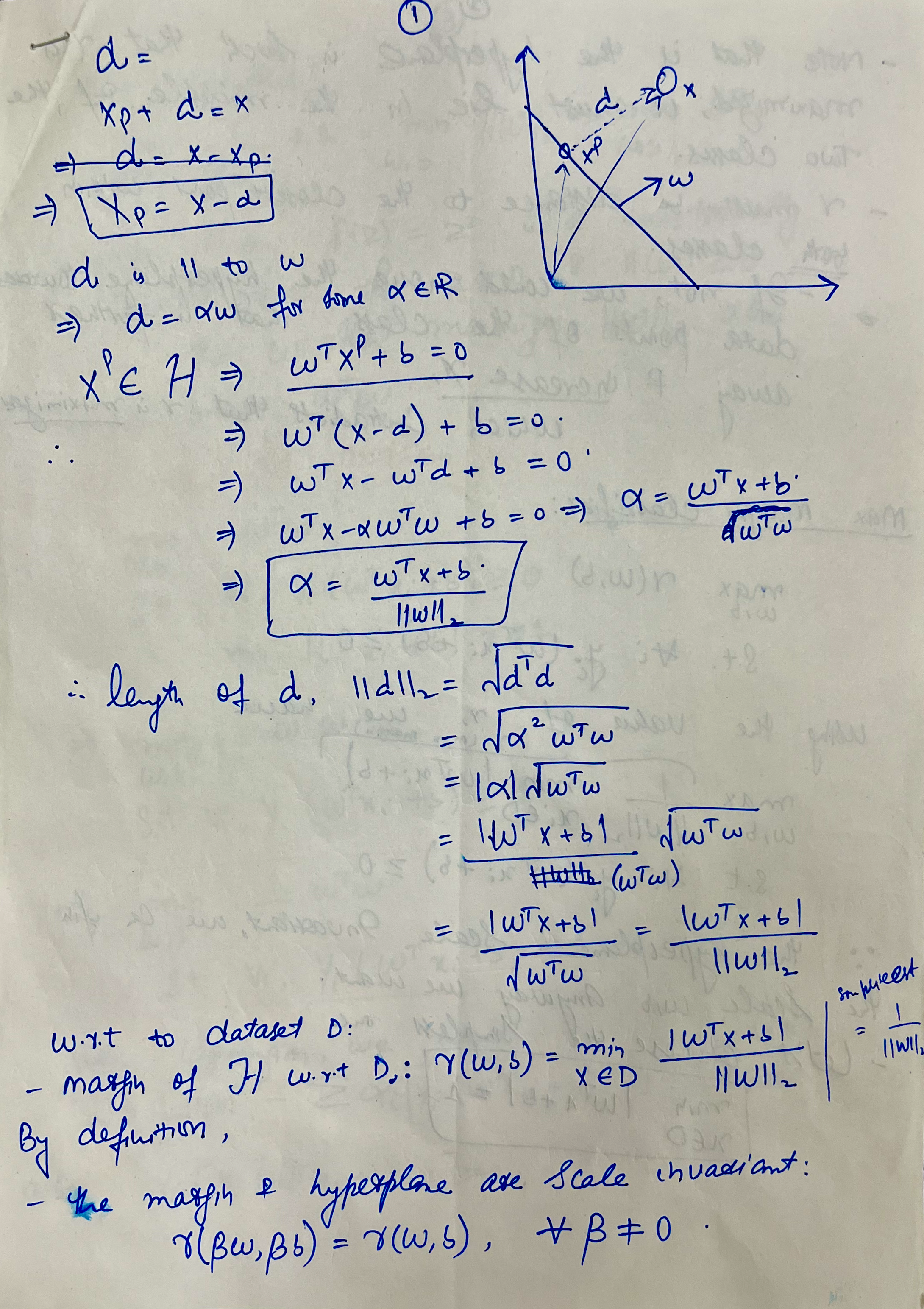
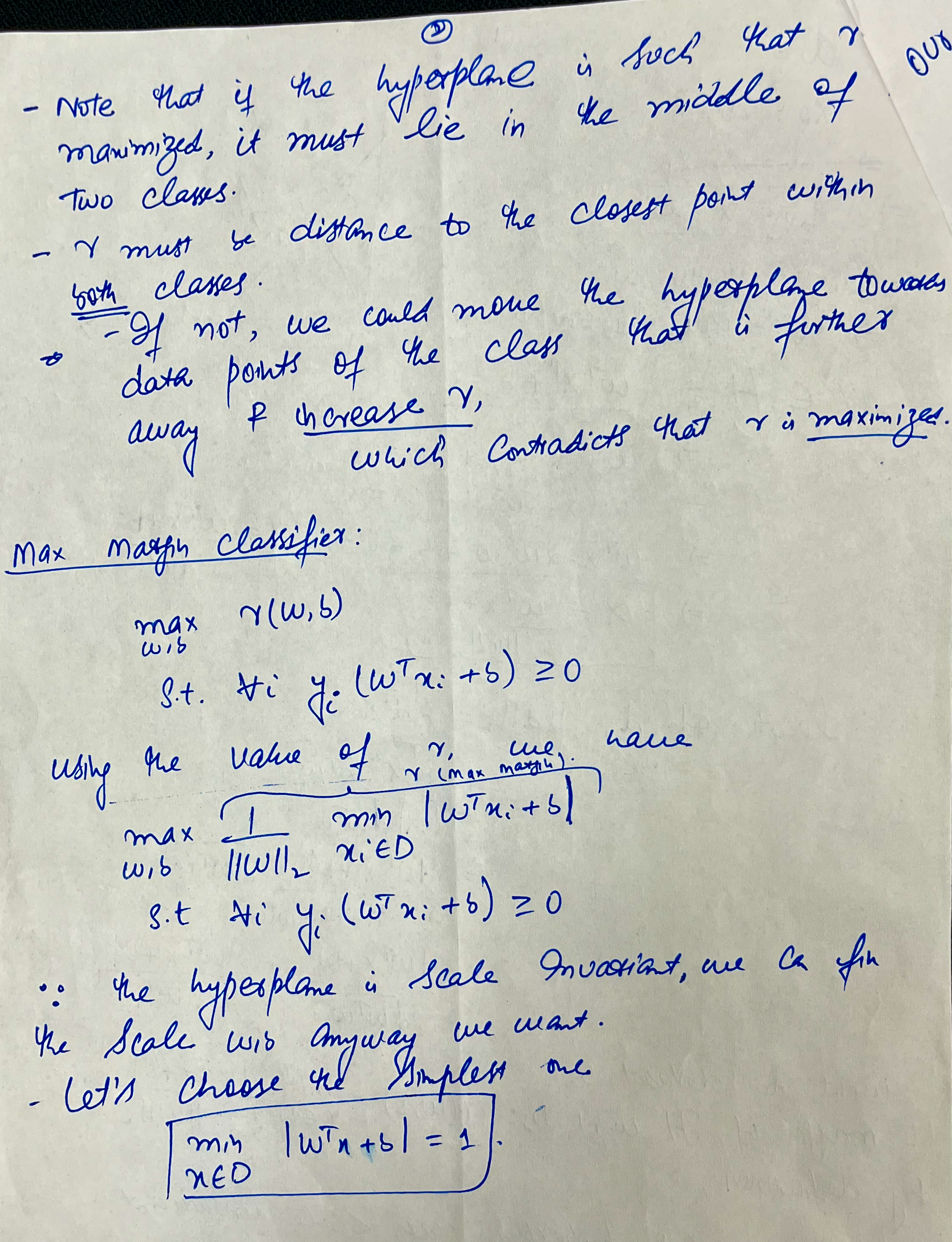
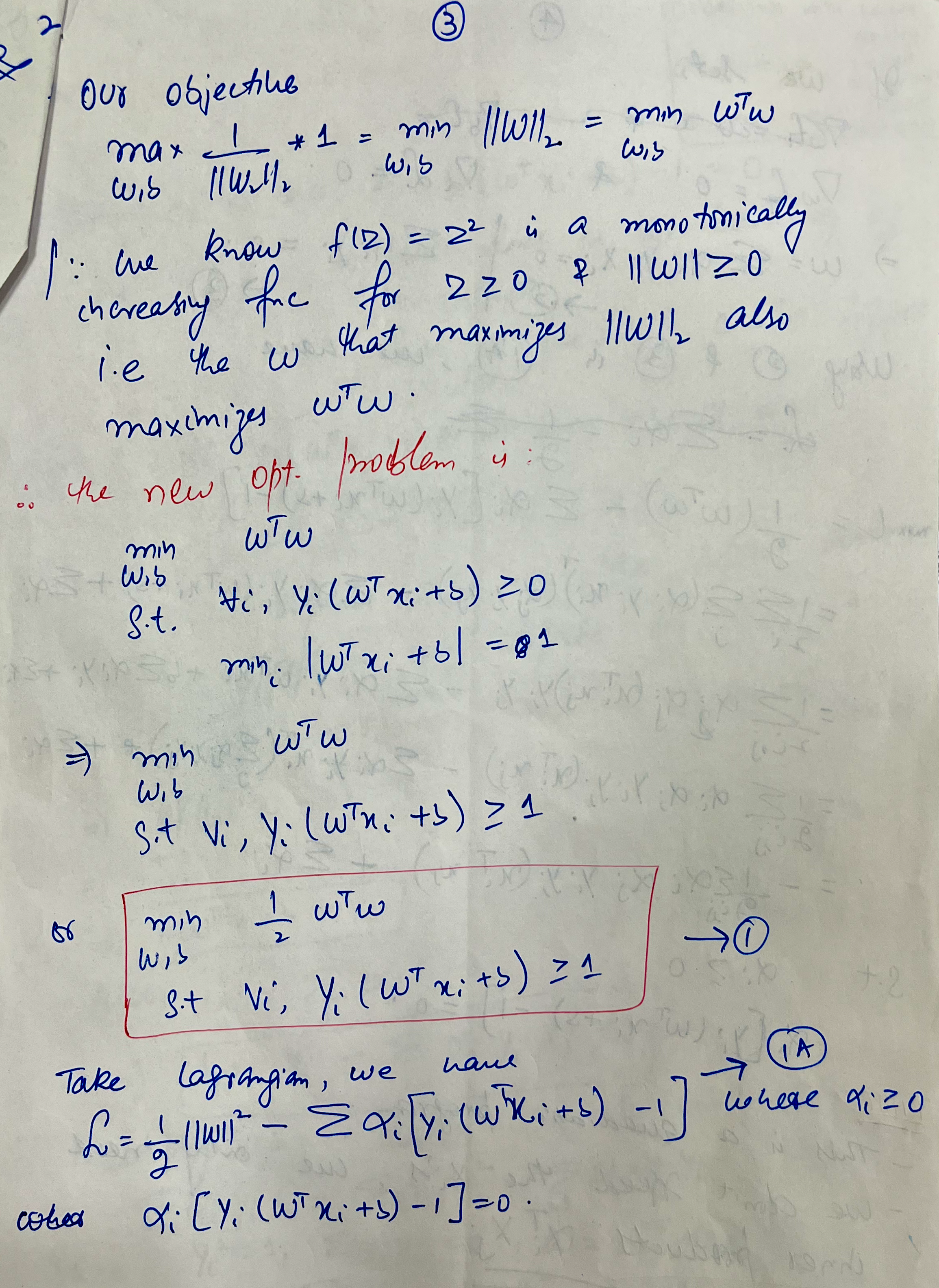
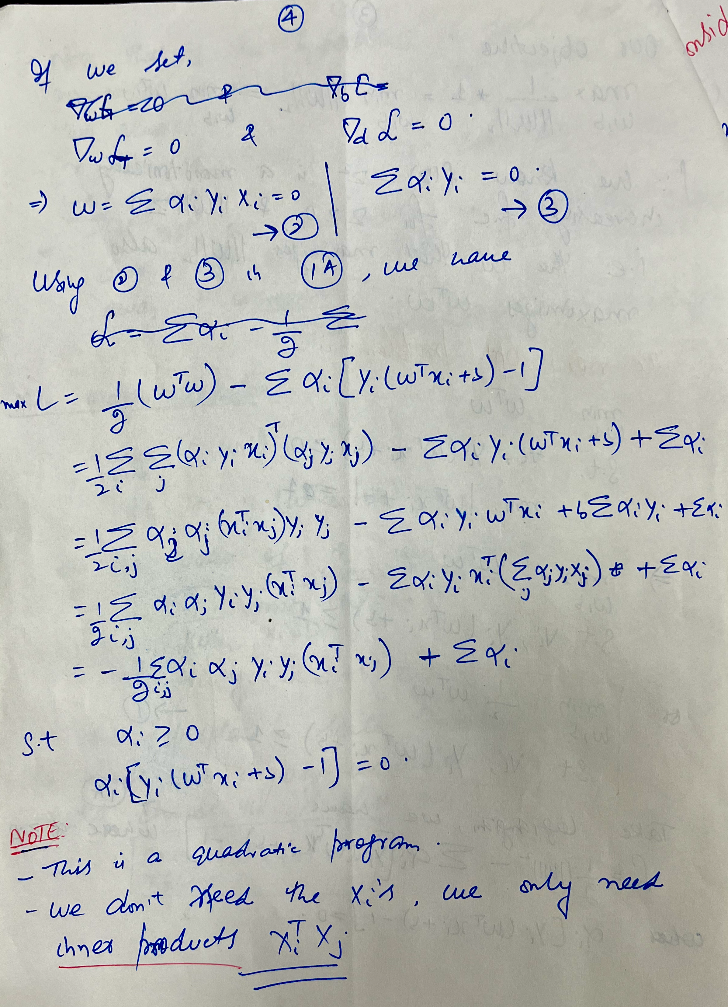
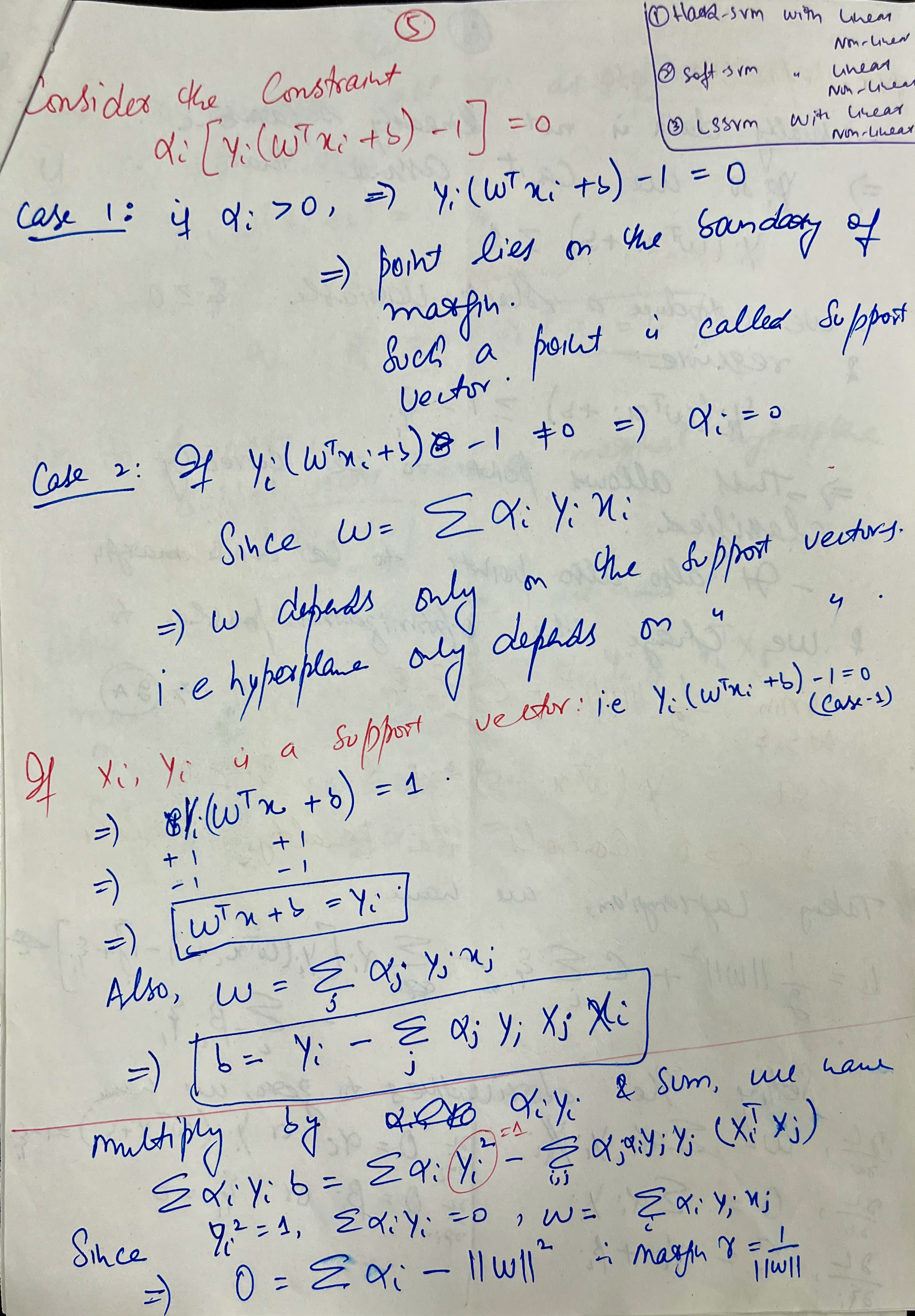
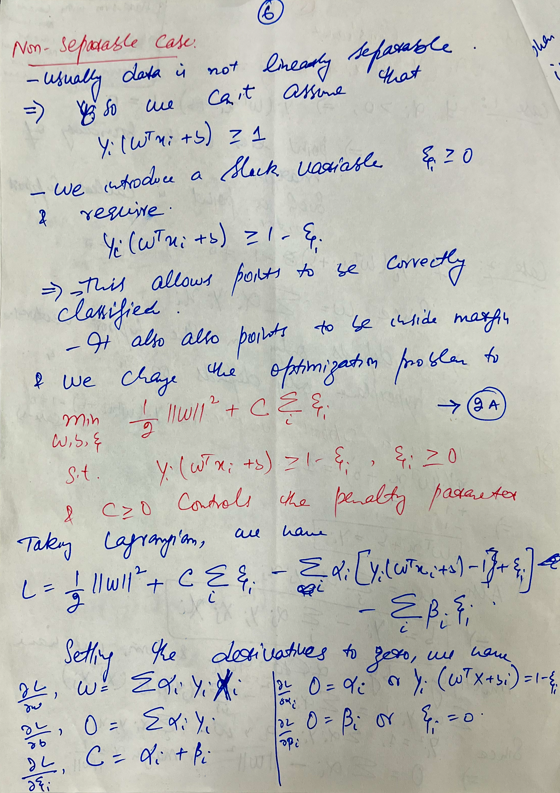
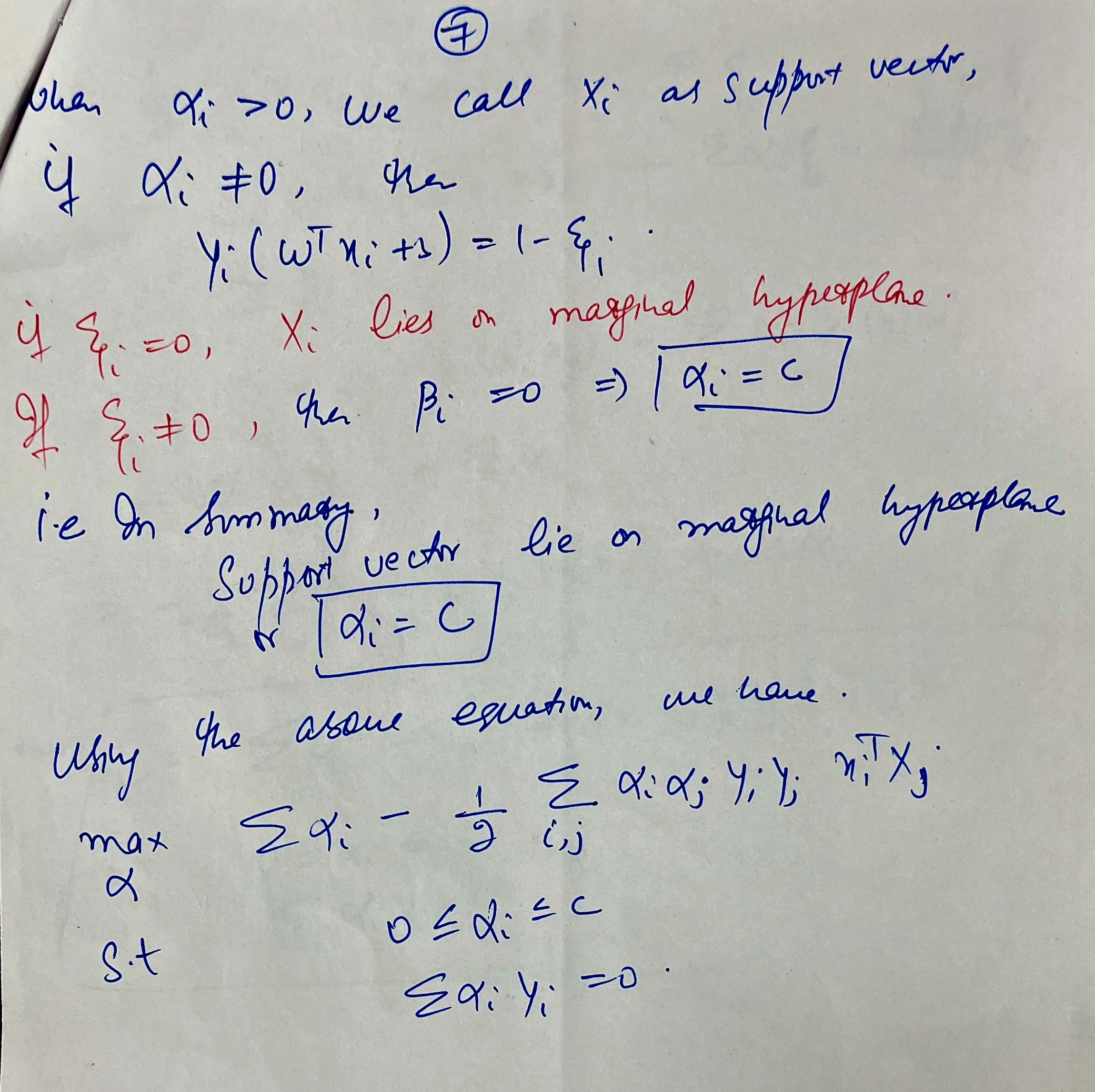
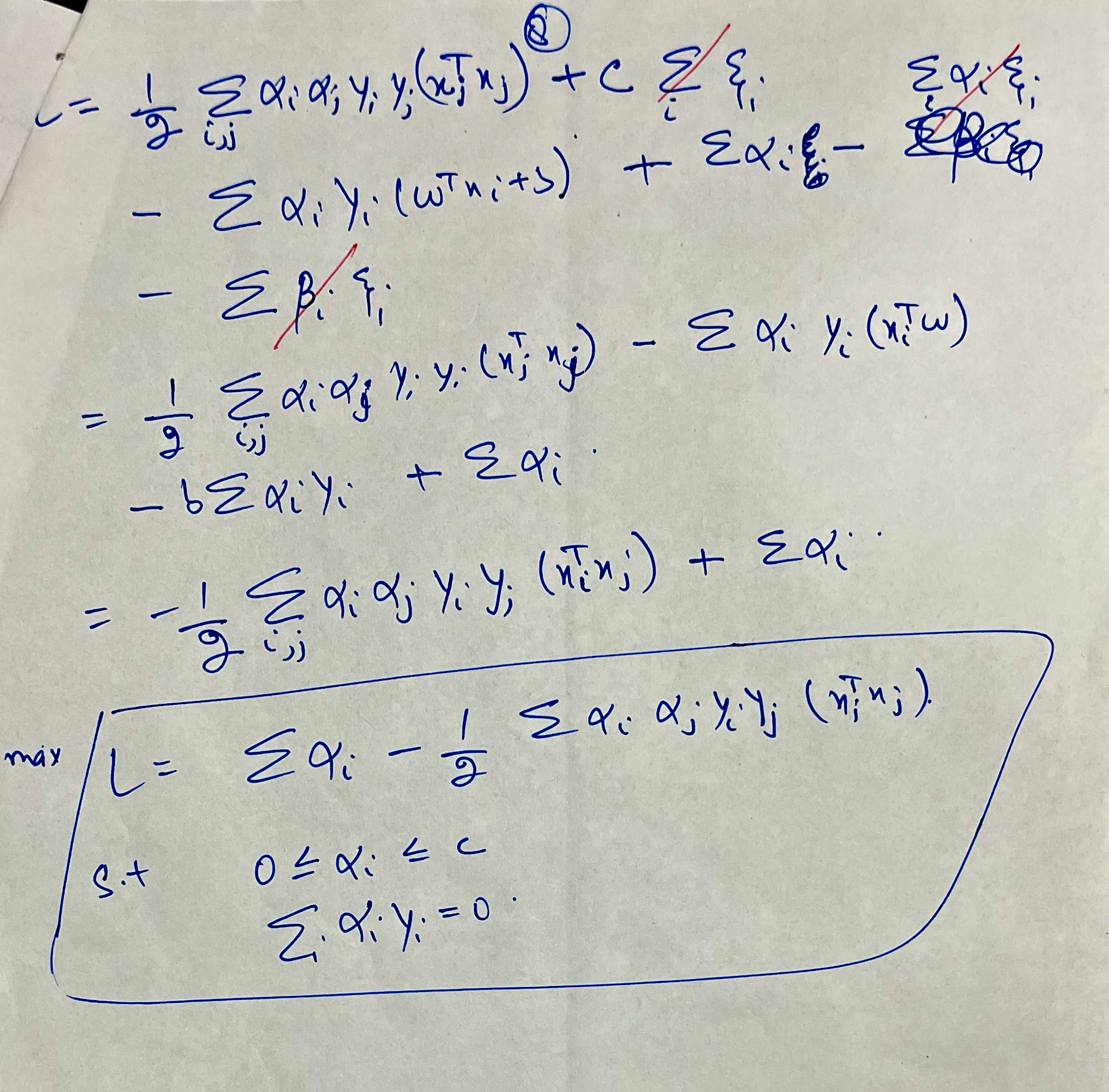
Notes by Dr. Mudasir Ahmad Sir suggested the following paper for further understanding: https://www.researchgate.net/publication/220578095_Least_Squares_Support_Vector_Machine_Classifiers
Introduction to Clustering
Overview of Clustering in Unsupervised Learning
Context of Clustering
In this lecture, clustering is introduced as a key method in unsupervised learning. Unlike representation learning, which includes techniques like Principal Component Analysis (PCA) and its variant Kernel PCA, clustering is aimed at discovering inherent group structures within a dataset.
Motivation for Clustering: Example
Consider a set of 2D data points scattered across three distinct regions. Here, PCA would capture variance along the main directions of the dataset, but it would miss local groups or clusters among the points. Clustering addresses this by grouping similar data points, aiming to capture more than variance alone.
Mathematical Notation
- Let the data points be represented by \(X = \{x_1, x_2, \dots, x_n\}\), where \(x_i \in \mathbb{R}^d\).
- We aim to partition this dataset \(X\) into \(k\) clusters.
Approaches and Definitions
Defining Clusters Using a Performance Metric
The clustering process involves assigning data points to clusters, aiming for homogeneity within each cluster. Formally, we define:
- Cluster Indicator Variable \(z_i\): For each data point \(x_i\), \(z_i \in \{1, 2, \dots, k\}\) denotes the cluster assignment.
- Cluster Centers (Centroids) \(\mu_k\): For each cluster \(k\), the center \(\mu_k\) is computed as the mean of all points assigned to that cluster.
Measuring Cluster Homogeneity
A common measure of clustering quality is the sum of squared distances (SSD) between each point and its cluster center, formulated as:
\[J = \sum_{i=1}^n \| x_i - \mu_{z_i} \|^2\]This expression minimizes within-cluster variance, making clusters as tight as possible.
The Clustering Problem and its Complexity
Combinatorial Complexity
Given \(n\) points and \(k\) clusters, the number of ways to partition \(X\) into \(k\) clusters grows exponentially. For instance, with \(n = 5\) points and \(k = 3\), there are \(3^5 = 243\) possible partitions.
NP-Hard Nature of Clustering
Finding the optimal partition requires testing all possible assignments, a task that is NP-hard. For a large number of points and clusters, the number of possible partitions becomes computationally infeasible, even for moderate values like \(n = 1000\) and \(k = 2\), leading to \(2^{1000}\) combinations.
Practical Solution: Heuristic Approaches
Since exact computation is infeasible, clustering typically relies on heuristic algorithms. The lecture hints at introducing a popular clustering heuristic, which will aim to minimize the partition cost \(J\) through an approximate solution.
Example: K-Means Objective Function
The K-Means algorithm is one such heuristic that iteratively refines cluster assignments and centers to reduce the SSD. Each iteration involves two main steps:
- Assignment Step: Assign each \(x_i\) to the nearest cluster center.
- Update Step: Recompute \(\mu_k\) as the mean of all points assigned to cluster \(k\).
The process continues until the SSD cost function \(J\) converges or a predefined number of iterations is reached.
Visual Illustration of Clustering Concepts
- Data Scatter Plot: The initial data points, grouped loosely across a 2D space, show an apparent need for clustering.
- Principal Component Line: A line representing the maximum variance (principal component) is drawn, showing how PCA might miss sub-group structures.
- Cluster Boundaries: Overlaying the plot with cluster boundaries or centroids illustrates the captured structure through clustering. Each point’s distance to its centroid demonstrates the optimization goal of minimizing this SSD distance.
Key Takeaways
- Clustering reveals structural relationships within data beyond simple variance.
- The process is complex due to its NP-hard nature, requiring heuristic approaches like K-Means for practical applications.
- Performance measures such as within-cluster sum of squared distances guide the quality of clustering results.
These notes cover clustering’s mathematical foundations, complexity considerations, and visual interpretations that clarify its role in unsupervised learning.
K-Means Clustering and Lloyd’s Algorithm
Overview of Lloyd’s Algorithm
Context and Terminology
This lecture introduces Lloyd’s Algorithm, commonly called the K-Means Algorithm, a popular approach to clustering in unsupervised learning. The objective of the K-Means problem is to partition a dataset into \(k\) clusters, each represented by a central point or “mean.” Lloyd’s algorithm iteratively approximates a solution to this problem.
Steps of Lloyd’s Algorithm
Step 1: Initialization
To begin clustering, we assign each data point a cluster indicator \(z\) as an initial label. This initialization step can be arbitrary but affects the final result and convergence speed. Each data point \(x_i\) is assigned a random \(z_i \in \{1, \dots, k\}\) that identifies its initial cluster.
Step 2: Compute the Mean (Centroid)
In each iteration, for every cluster \(k\), calculate the centroid \(\mu_k\) by averaging the data points assigned to it. This centroid update for each cluster \(k\) can be expressed as:
\[\mu_k^{(t)} = \frac{1}{|C_k|} \sum_{x_i \in C_k} x_i\]where \(C_k\) is the set of all data points currently assigned to cluster \(k\).
Step 3: Reassignment Step
After updating centroids, each data point ( x_i ) is reassigned to the cluster with the nearest mean. The cluster indicator \(z_i\) is updated as:
\[z_i = \underset{k}{\operatorname{arg\,min}} \| x_i - \mu_k^{(t)} \|^2\]This step ensures that each point moves towards the cluster that minimizes its distance to the centroid.
Convergence and Termination
Convergence Criteria
The algorithm iterates until convergence, defined as a state where no points change clusters. This can occur when each point’s distance to its current cluster centroid is less than or equal to the distance to any other centroid.
- Convergence Check: If, in a given iteration, no points are reassigned to different clusters, the algorithm terminates.
- Loop Prevention: Lloyd’s algorithm avoids infinite loops by consistently reducing the sum of squared errors (SSE) with each iteration. Thus, convergence is guaranteed, although it may not always reach the global optimum.
Potential Limitations
While Lloyd’s algorithm is guaranteed to converge, it may not find the optimal clustering. The converged solution can depend heavily on the initialization and might only be a local minimum. This limitation is a trade-off due to the problem’s NP-hard nature.
Example Walkthrough: A K-Means Cycle
- Initialize clusters: Randomly assign data points to initial clusters.
- Compute Centroids: Calculate centroids for each cluster based on current assignments.
- Reassign Points: Reassign each data point to the closest centroid.
- Repeat: Continue the compute-reassign cycle until convergence.
This process illustrates how points iteratively move closer to centroids, forming tight clusters.
Key Questions on Lloyd’s Algorithm
Q1: Does the Algorithm Converge?
Yes, Lloyd’s algorithm is proven to converge since it decreases the SSE in each iteration. However, convergence depends on the initialization and may lead to suboptimal clusters.
Q2: What Kind of Clusters Does It Produce?
Lloyd’s algorithm tends to create compact, spherical clusters but may struggle with datasets that have varying densities or non-spherical shapes.
Q3: How Should Initialization Be Performed?
Initialization can impact results significantly. Common techniques include random selection or methods like K-Means++ for smarter initial placement of centroids to improve convergence quality.
Q4: How Do We Choose \(k\)?
The number of clusters \(k\) is often unknown and determined by evaluation metrics like the Elbow Method or Silhouette Score to assess the best number of clusters based on dataset characteristics.
Key Takeaways
- Lloyd’s algorithm is a popular heuristic for clustering, especially useful for quick approximations.
- Despite limitations like sensitivity to initialization and local minima, it produces reasonable clusters in practice.
- Selecting \(k\) and initializing centroids are key to improving the performance of the algorithm.
These notes cover Lloyd’s algorithm’s steps, convergence properties, and practical considerations for clustering.
Convergence of the K-Means Algorithm
Introduction to K-Means Convergence
Overview
This lecture delves into the convergence properties of Lloyd’s Algorithm (often known as the K-Means Algorithm) for clustering, specifically answering whether and how this algorithm reaches a stable state where no further cluster reassignments are necessary.
Key Questions on Convergence
- Does the Lloyd’s Algorithm converge?
- If it converges, what type of clusters does it produce?
- What effect does initialization have on the clustering results?
- How should we choose the number of clusters, \(k\)?
This session primarily focuses on the first question: proving that Lloyd’s Algorithm does indeed converge.
Mathematical Proof of Convergence
Step 1: Establishing the Objective Function
The objective function \(J\) is defined as the sum of squared Euclidean distances from each point to its cluster centroid. For a given set of cluster assignments, \(J\) is calculated as:
\[J = \sum_{i=1}^{n} \| x_i - \mu_{z_i} \|^2\]where \(\mu_{z_i}\) is the centroid of the cluster that data point \(x_i\) is currently assigned to.
Step 2: Iterative Reassignment
In each iteration, the algorithm performs two main steps:
-
Update Centroids: Calculate new centroids \(\mu_k\) for each cluster. \(\mu_k = \frac{1}{|C_k|} \sum_{x_i \in C_k} x_i\) where \(C_k\) is the set of all data points currently assigned to cluster \(k\).
-
Reassign Points: For each point \(x_i\), update its cluster assignment \(z_i\) to the nearest centroid: \(z_i = \underset{k}{\operatorname{arg\,min}} \| x_i - \mu_k \|^2\)
Step 3: Reduction of the Objective Function
Each reassignment strictly reduces the objective function \(J\). This is due to a fundamental property of Euclidean distance: the sum of squared distances of points to their own cluster’s centroid is minimized when points are assigned to the nearest centroid.
Step 4: Finite Number of Partitions
Since there are only a finite number of possible cluster assignments, the algorithm must eventually reach a state where no further improvements (reassignments) are possible, thus leading to convergence.
Key Insight: Why Convergence Happens
The convergence of the Lloyd’s Algorithm is based on two core ideas:
- Objective Function Minimization: With each iteration, \(J\) decreases, ensuring that the algorithm does not revisit previous partitions.
- Finite Partition Possibilities: There is a finite number of ways to partition \(n\) data points into \(k\) clusters, so continual reassignment cannot go on indefinitely.
Implications of Convergence
- Local Minima: Convergence does not guarantee the global minimum of the objective function. The solution reached is often a local minimum, influenced by the initial cluster assignments.
- Algorithm Performance: Although convergence is guaranteed, the rate of convergence depends on factors such as data distribution and the initial positions of centroids.
Summary of the Convergence Proof
In summary, Lloyd’s Algorithm will always converge, but the result may depend on initialization and may not provide the globally optimal clustering configuration.
Nature of Clusters Produced by K-Means
Introduction
This lecture examines the types of clusters formed by the K-Means Algorithm (Lloyd’s Algorithm) and explores the geometric structure of these clusters. Specifically, it discusses the characteristics of clusters produced when using the K-Means algorithm and how the resulting clusters align with the mathematical concept of Voronoi regions.
Geometric Structure of K-Means Clusters
Simple Case: \(k = 2\)
- Two Cluster Centers: Consider a scenario where the data is divided into two clusters with centroids (means) labeled as \(\mu_1\) and \(\mu_2\).
-
Partition Condition: For a point \(x\) in cluster 1, the distance from \(x\) to \(\mu_1\) must be less than or equal to the distance to \(\mu_2\). Mathematically, this condition is expressed as:
\[\| x - \mu_1 \|^2 \leq \| x - \mu_2 \|^2\]Simplifying, we find that the region dividing the data between clusters 1 and 2 is defined by:
\[x^T (\mu_2 - \mu_1) \leq \frac{\|\mu_2\|^2 - \|\mu_1\|^2}{2}\]This expression represents a linear boundary (hyperplane) between the two clusters, implying that the data space is divided into two regions by this boundary, with each region corresponding to a cluster.
Generalization to \(k = 3\)
When three clusters \(\mu_1\), \(\mu_2\), and \(\mu_3\) are present:
- Three Pairwise Boundaries: Similar to the two-cluster case, boundaries are formed between each pair of centroids, resulting in three dividing hyperplanes.
- Intersection of Regions: Points are assigned to cluster 1 if they are closer to \(\mu_1\) than to \(\mu_2\) or \(\mu_3\). This results in regions that are intersections of the half-spaces defined by the dividing hyperplanes.
The general shape formed by this arrangement is known as a Voronoi region, where each cluster’s region is the space closer to its centroid than any other.
Voronoi Regions and High Dimensions
- Voronoi Definition: A Voronoi region for a centroid \(\mu_k\) is the set of all points in space that are closer to \(\mu_k\) than to any other centroid.
- High-Dimensional Implication: In higher dimensions, each cluster’s region is still defined by intersecting half-spaces. Thus, in \(d\)-dimensional space, each cluster region resembles a higher-dimensional Voronoi cell, maintaining the concept of proximity-based partitions.
Limitations of K-Means with Non-Linear Boundaries
The K-Means Algorithm can struggle with data that does not conform to Voronoi-like boundaries, such as concentric circles. In these cases:
- Linear Boundary Issue: K-Means will only produce clusters separated by linear boundaries. As a result, it cannot accurately separate points in concentric clusters using linear boundaries alone.
- Kernelized K-Means: To handle non-linear structures, Kernel K-Means maps data into a higher-dimensional space, allowing for more flexible, non-linear partitions.
Summary of Cluster Characteristics
- Linear Separators: K-Means clusters are separated by linear boundaries, making them ideal for data that aligns well with such partitioning.
- Voronoi-Based Partitioning: K-Means creates clusters that correspond to Voronoi regions, with each cluster encompassing points closer to its centroid than to any other.
- Handling Complex Structures: Kernel methods, such as Kernel K-Means, offer extensions to address data with non-linear separations.
Initialization of Centroids in K-Means and K-Means++
Introduction
This lecture focuses on initialization methods for centroids in the K-Means algorithm, especially exploring how initialization can impact the quality and efficiency of clustering. The K-Means++ initialization is introduced as a more sophisticated approach, aiming to enhance cluster quality by spacing out initial centroids.
Basic Initialization Approaches
Uniform Random Initialization
- Random Assignment: One straightforward method is to initialize by randomly assigning points to clusters.
- Uniformly Select Centroids: Another common approach is to select \(k\) random points as initial centroids from the dataset. For example, if the dataset has 1000 points and \(k = 5\), then five points are selected at random, each representing a cluster.
This random initialization guarantees convergence but may lead to poor clustering outcomes due to local minima.
K-Means++ Initialization
Overview of K-Means++ Strategy
K-Means++ improves upon random initialization by spreading out the centroids as much as possible, thereby enhancing the likelihood of reaching a better clustering solution. The goal is to place each new centroid farthest from the previously chosen centroids, ensuring that each centroid represents a distinct portion of the data.
Step-by-Step K-Means++ Initialization
- Choose the First Centroid: Select the first centroid \(\mu_1\) uniformly at random from the data points.
- Iteratively Select Subsequent Centroids:
- For each new centroid \(\mu_l\) where \(l = 2, \dots, k\), calculate a score for each remaining point based on its distance to the nearest chosen centroid.
-
Define the score for each point \(x\) as:
\[\text{score}(x) = \min_{j \in \{1, \dots, l-1\}} \| x - \mu_j \|^2\]
-
Select Probabilistically: Choose the next centroid with a probability proportional to its score. Points farther from existing centroids have a higher probability of being chosen, encouraging more spread-out clusters.
- Repeat: Continue until \(k\) centroids are selected.
Advantages of K-Means++ Initialization
- Better Objective Value: K-Means++ tends to yield a lower sum of squared distances than random initialization.
- Theoretical Guarantee: The K-Means++ initialization ensures that the objective function is within a factor of 2 (or less) of the optimal solution on average, which is a significant improvement over random initialization.
Mathematical Guarantee of K-Means++
K-Means++ initialization provides a probabilistic guarantee for the objective function \(J\), where \(J\) is defined as:
\[J = \sum_{i=1}^n \| x_i - \mu_{z_i} \|^2\]where \(z_i\) represents the cluster assignment of point \(x_i\), and \(\mu_{z_i}\) is the centroid of cluster \(z_i\).
For the best possible partition, the minimized objective function is:
\[\min_{z} \sum_{i=1}^n \| x_i - \mu_{z_i} \|^2\]K-Means++ guarantees that the expected objective function after initialization and clustering will not exceed a constant multiple of the optimal objective value, typically within a factor of O(log k) of the best possible solution.
Summary
- Random Initialization is simple but can lead to suboptimal clusters.
- K-Means++ Initialization improves centroid placement by spacing centroids, increasing the likelihood of achieving high-quality clusters.
- Theoretical Guarantee: K-Means++ offers a bound on the objective function, ensuring more reliable clustering results.
Choosing the Number of Clusters \(K\) in K-Means
Introduction
In clustering tasks using the K-Means algorithm, the choice of \(K\) (the number of clusters) significantly impacts the quality of clustering. Since \(K\) is often not known in advance, this lecture outlines heuristic methods to determine an optimal \(K\), balancing the objective function value and penalizing excessive cluster numbers.
Objective Function in K-Means
The objective function in K-Means is defined as the sum of squared distances from each point to its assigned cluster center. Formally, for a given set of clusters \(\{z_1, \dots, z_n\}\):
\[f(z_1, \dots, z_n) = \sum_{i=1}^n \| x_i - \mu_{z_i} \|^2\]where \(\mu_{z_i}\) is the centroid of the cluster to which point \(x_i\) belongs. Lower objective values indicate tighter clusters, but without a penalty, setting \(K = n\) minimizes the objective function to zero, which is trivial and uninformative.
Balancing Objective and Penalty
To prevent choosing a trivially high \(K\), a penalty for the number of clusters is introduced. Thus, the total function to minimize becomes:
\[\text{Total Objective} = \text{Objective Value} + \text{Penalty for K}\]The penalty function increases with \(K\), discouraging excessive clusters. A good choice for \(K\) minimizes this combined metric, achieving balance between minimizing the objective value and not using too many clusters.
Visualizing the Trade-Off: Objective vs. Penalty
A plot of Objective Value + Penalty against \(K\) typically shows a decreasing trend initially, where adding clusters reduces the objective significantly. However, as \(K\) grows, the penalty overtakes the gains in clustering quality, and the total cost starts to increase. The optimal \(K\) is where the total cost reaches its minimum, denoted by \(K^*\).
Common Methods for Choosing \(K\)
1. AIC (Akaike Information Criterion)
The AIC criterion for determining \(K\) combines the objective value with a linear penalty on \(K\):
This method penalizes larger \(K\), helping select a model that balances complexity and fit to the data.
2. BIC (Bayesian Information Criterion)
The BIC criterion introduces a logarithmic dependency on \(n\) (number of data points) along with \(K\):
The BIC criterion assumes a probabilistic model of data generation, offering a more conservative penalty for large datasets by favoring smaller \(K\) values.
3. Elbow Method
The Elbow Method involves plotting the objective value against \(K\) and identifying the point where additional clusters result in diminishing improvements, creating an “elbow” shape. This elbow indicates the optimal \(K\) where adding clusters yields minimal gains in clustering quality.
Summary
- Objective Function: Minimizing the sum of squared distances alone encourages high \(K\) but does not provide meaningful clusters.
- Penalization: A penalty for \(K\) helps balance cluster compactness with a manageable number of clusters.
- Heuristic Methods: Methods like AIC, BIC, and the Elbow Method assist in determining an effective \(K\), using a blend of statistical modeling and visualization.
Learning From Data
Lady Tasting Tea
The “Lady Tasting Tea” experiment is a famous example in the history of statistics, conducted by the British statistician and geneticist Ronald A. Fisher in the 1920s. This experiment was designed to test whether a woman, referred to as “the lady,” could distinguish between two methods of making tea. Specifically, she claimed that she could tell whether milk was added to the cup before or after the tea. Fisher’s experiment was one of the first to rigorously apply principles of experimental design and statistical inference, and it laid foundational ideas in hypothesis testing.
Here’s a breakdown of the experiment and its significance:
1. The Claim The lady claimed that she could taste the difference between tea prepared with milk added first and tea prepared with tea added first.
2. The Experiment Setup To test her claim, Fisher designed an experiment where the lady was given eight cups of tea. Four cups had milk added first, and four had tea added first, but she did not know which were which.
3. Hypotheses Fisher set up two hypotheses:
- Null Hypothesis (H0): The lady cannot distinguish between the two types of tea (any correct guesses would be due to chance).
- Alternative Hypothesis (H1): The lady can distinguish between the two types of tea better than random chance.
4. Randomization and Control To prevent bias, the order in which the cups were presented to the lady was randomized, and she had to identify which cups were which based purely on taste, with no other clues or hints.
5. Statistical Test and Decision The lady then attempted to classify each cup correctly. Fisher used a combinatorial analysis to calculate the probability of her guessing the cups correctly purely by chance. If she identified all cups correctly, Fisher reasoned that this outcome would be unlikely under the null hypothesis (i.e., if she were just guessing). This would provide evidence that she indeed had the ability to taste the difference.
6. Fisher’s Exact Test From this experiment, Fisher developed what we now call “Fisher’s Exact Test,” a statistical test used to determine if there are nonrandom associations between two categorical variables, particularly in small sample sizes.
Significance of the Experiment The “Lady Tasting Tea” experiment illustrated some core principles of modern statistical testing:
- Hypothesis Testing: Formulating and testing a null hypothesis against observed data.
- P-value Concept: Estimating the probability of an observed result under the null hypothesis.
- Experimental Design: Fisher emphasized the importance of randomization and control to avoid bias.
This experiment is now widely taught as a fundamental example in statistics, as it elegantly captures the essence of hypothesis testing and the use of probability to make inferences in experiments.
The conclusion of the “Lady Tasting Tea” experiment was that the lady in question was indeed able to identify the difference between the two methods of adding milk (milk-first vs. tea-first) with greater accuracy than would be expected by chance. Fisher’s experiment showed that the probability of her guessing correctly by chance was low enough to reject the null hypothesis. This provided evidence that she could indeed distinguish between the two methods, suggesting that the taste difference was real and perceptible for her, at least under the controlled conditions of the experiment.
Neural Networks


Lecture-11/11/2024
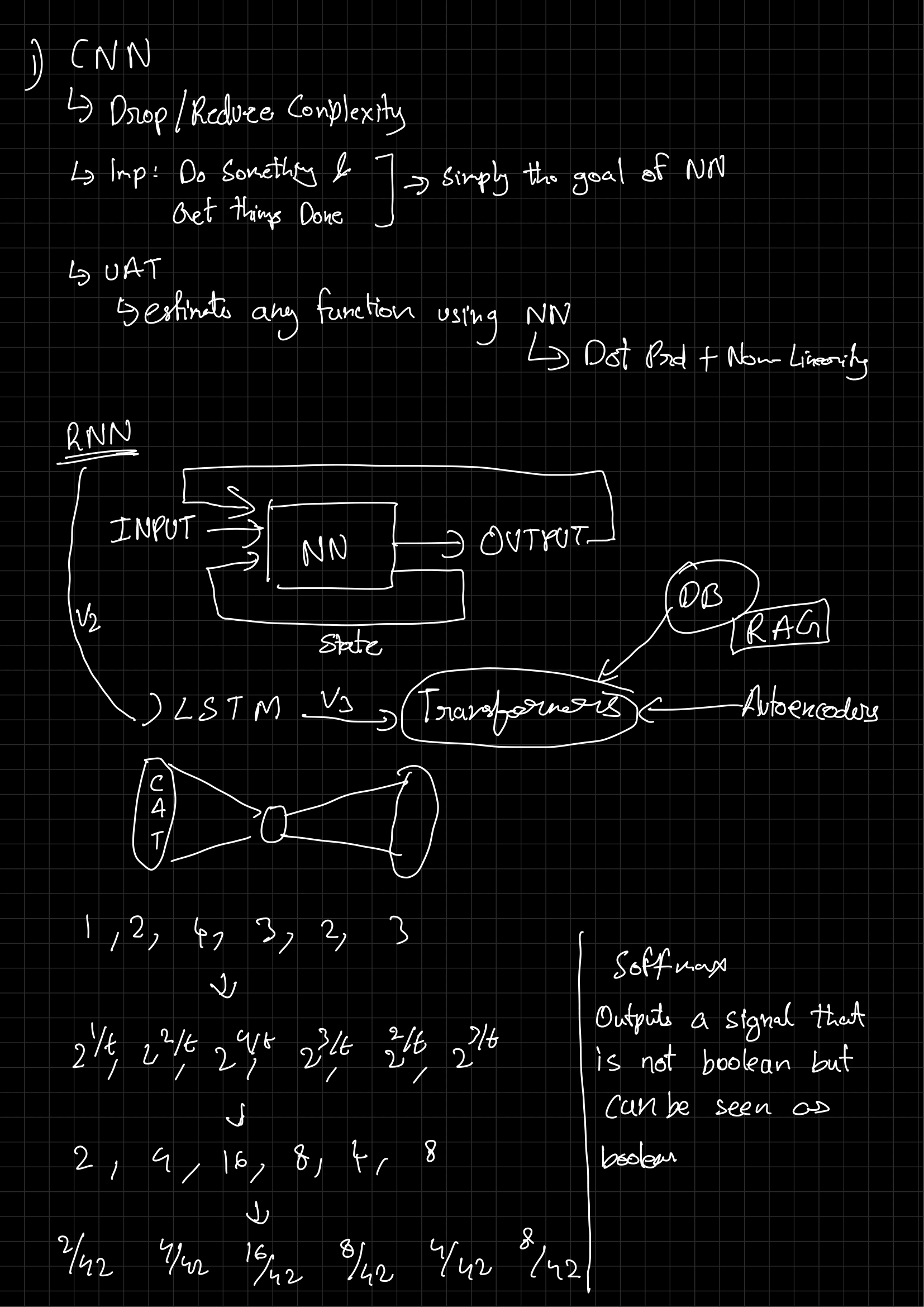
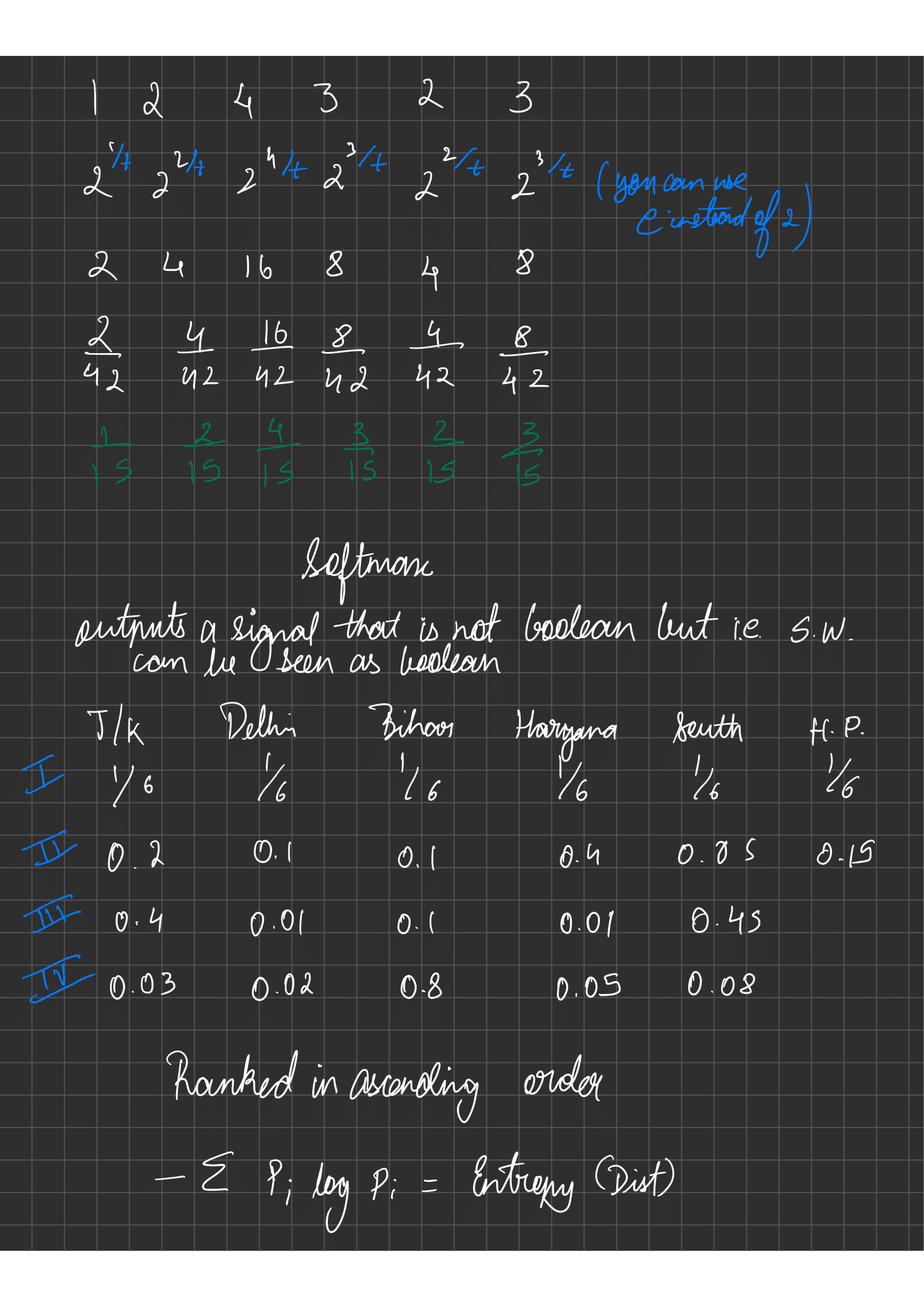
First draft notes by Aashik Arun Bobade. For any corrections, contact: bobadeaashik@gmail.com.